Data Models for Self-Service BI

The self-service BI journey starts with the business user importing data. With Microsoft Power Pivot, we encourage the user to import tables and create relationships among these tables, similar to what they would do with Microsoft Access. This brings tremendous flexibility because it allows the user to incrementally add new datasets and implement sophisticated models for consolidated reporting, such as for analyzing reseller and internet sales side by side. True, Power Pivot relationships have limitations, including:

  • The lookup table must have a primary key and the relationship must be established using this key. As it stands, Power Pivot doesn’t support multi-grain relationship where the fact table joins the lookup table at a higher grain than the primary key.
  • Many-to-many relationships (such as a joint bank account) are not natively supported and currently require simple DAX formulas to resolve the relationship, such as CALCULATE ( SUM ( Table[Column] ), BridgeTable)
  • Closed loop relationships (Customer->Sales->Orders->Customer) are not allowed, etc.

The chances that these constraints will be relaxed in time as Power Pivot and Tabular evolve to allow you to meet even more involved requirements on a par with organizational BI models.

033014_1952_DataModelsf1

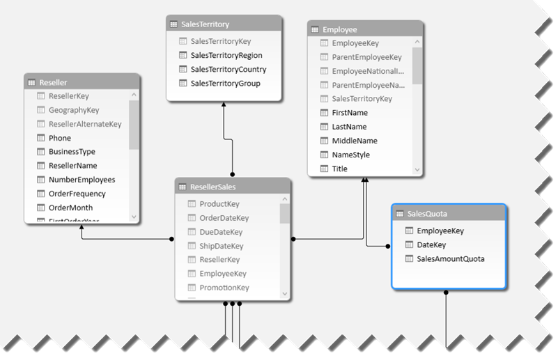
With the recent popularity of other tools for self-service BI tools, I took a closer look at their data features. Tableau, for example, encourages users to work with a single dataset. If the user wants to import data from multiple tables, the user must create table joins to relate the tables before data is imported in order to create a dataset that has all the required data. This probably meets 80% of self-service BI requirements out there although it might preclude consolidated analysis. Suppose you want to analyze reseller sales by customer. With Tableau, you need to join the Customer and ResellerSales tables in order to prepare the dataset and that’s probably OK to meet this requirement. At some point, however, suppose you need to bring also Internet sales which are stored in a separate table. Now you have an issue. If you opt to change the dataset and join the Customer, ResellerSales, and InternetSales, you’ll end up with duplicated data because you can’t join ResellerSales to InternetSales (they don’t have a common field). In Power Pivot, you could simply address this by importing Customers, ResellerSales, and InternetSales as separate tables and creating two relationships Customer->ResellerSales and Customer->InternetSales. Notice that a Power Pivot relationship happens after the tables are imported although it’s possible of course to establish a data source join during the data import. A Tableau workaround for the above scenario would be to go for “data blending”. Speaking of which…

It’s also interesting how Tableau addresses combining data from separate data sources. Referred to as “data blending”, this scenario requires the user to designate one of the data sources as primary and specifying matching fields from the two data sources to perform the join. Behind the scenes, Tableau executes a post-aggregate join that aggregates data at the required grain. Let’s say, you import the Customer table from Data Source A and InternetSales table from Data Source B. Suppose that both the Customer and InternetSales datasets have a State field which you want to use for the join. With data blending, Tableau will first aggregate the InternetSales dataset at the State level (think of SUM(SALES) FROM … GROUP by STATE) and then join this dataset to the Customer dataset on the State field. The advantage of this approach is that you can join any two datasets as long as they have a common field (there is no need for a primary key in the Customer table). The disadvantage is that the secondary data source can’t be joined to another (third) data source. Further, this approach precludes more complicated data entity relationships, such as many-to-many.

When choosing a self-service BI tool, you need to carefully evaluate features and one of the most important criteria is the tool data capabilities. Some tools are designed for one-off analysis on top of a single dataset and might require importing the same data to meet different reporting requirements. Power Pivot gives you more flexibility but requires end users to know more about data modeling, tables and relationships.


Building a Custom ETL Framework with SSIS 2012

Even though the SSIS catalog and the new project deployment mode in SQL Server 2012 take care of many of the mundane monitoring needs, a custom ETL framework is still important for handling features such as restartability and parallelism. Join our next Atlanta BI User Group meeting on Monday, March 31st when Aneel Ismaily will talk about this subject in his “Building a Custom ETL Framework with SSIS 2012” presentation.

“ETL Frameworks are the foundation of any data warehouse/data mart implementation. In this session we will discuss building a heavy-duty enterprise ETL Framework and will talk in detail about some major ETL enhancements available in SQL Server 2012. Topics include auditing, logging, designing for fault tolerance and recoverability, handling orchestration, parallelism and finally scheduling.”

X-IO will sponsor the meeting and present their Intelligent Storage Element fast storage product.

Dynamic Dimensions

Scenario

You need to assign a dimension dynamically to a cube measure group, such as to calculate binning. In the extreme example, you might need to perform fact row level evaluation to determine where the dimension “fits” in. Consider the following example from the insurance industry. An ODS-style Claim table interprets every change to the claim table as a Type 2 change by creating a new row and expiring the previous row of the claim.

Claim_KeyStart_DateEnd_DateClaim_NumberStatus
11/1/20105/1/2010C00001New
25/2/20103/8/2012C00001Open
33/9/201212/31/9999C00001Closed


Options

Given this scenario, you might want to count the number of claims as of any date. You have two options:

  1. Create a Claim Snapshot fact table taken at a daily or monthly interval.
  2. Dynamically associate the Date dimension. In Multidimensional, this will require creating a Claim dimension and a Claim measure group, both bound to the same Claim table. Then, you can use the following script to “associate” the Date dimension (added as a unrelated dimension to the cube) to the Claim measure group:

CREATE MEMBER CURRENTCUBE.[Measures].[ClosingAccountingDate] AS [Date].[Calendar].MemberValue, VISIBLE = 0 ;

Scope

(

(

MeasureGroupMeasures(“Fact Claim”)

{

[Measures].[Start Date],

[Measures].[End Date]

}

),

[Date].[Calendar].Members,

Leaves([Claim])

);

this = iif ([Measures].[ClosingAccountingDate]>=[Measures].[Start Date] and [Measures].[ClosingAccountingDate]<=[Measures].[End Date],

Measures.CurrentMember, null);

End Scope;

End Scope;

To simplify the evaluation, the MemberValue property of all attributes of the Date dimension is bound to the closing date of the period, e.g. 12/31/2014 for year 2014, 3/31/2014 for any day in Q1, and 1/31/2014 for any day in January 2014. The scope assignment includes all measures in the Fact Claim measure group, except the Start Date and End Date measures since we don’t want to overwrite them. It also scopes on all members of the Calendar hierarchy of the Date dimension so that the calculation is performed at any level of the Calendar hierarchy. For example, if the user selects 2014 as a year, the calculation is performed as of 12/31/2014. Moreover, the Leaves([Claim]) scope positions at the measure leaves so we can evaluate any row in the fact table by comparing if the ‘as of’ date falls in the range of Start Date and End Date for that row.

032314_2359_DynamicDime1

Are we happy? We might be but end users might not be so excited. The problem is that this remarkably simple scope assignment can put a remarkable dent in the query performance. For any date, the server has to perform the evaluation for every row in the fact table. With a Claim dimension and a measure group with 500,000 rows, calculating the counts executes relatively fast (within a few seconds). However, running a trend query that requests counts for every day in a quarter might take a minute or so. The larger the claim dimension and the cube subspace that the query requires, the worse the performance will be. The performance is further impacted if you have other calculations on top of the claim counts.

Scope assignments are a very powerful and useful feature of Multidimensional but you shouldn’t abuse them. Keep the scope as narrow of possible to limit the cube space where the calculation is applied. Although it might require ETL effort, materialize whenever you can. For example, although it might result in millions of rows, a snapshot would perform much better with the above scenario. Further, performance can be further enhanced by partitions and aggregations while dynamic granular calculations won’t.

KPIs on Smartphone

Some of your might be familiar with the PushBI mobile BI offering of Extended Results. The company was recently acquired by Tibco. Now rebranded as Tibco Spotfire Metrics, its mobile BI offering is now available for the most popular mobile platforms, including Windows Phone and Windows 8. As its documentation explains, Spotfire Metrics supports surfacing KPIs from a variety of data sources, including Analysis Services. If you’re looking for ways to present KPIs to mobile phones, Spotfire Metrics could fill in the gap.

030214_2329_KPIsonSmart1