Some of you have approach Geoff Hiten and me about forming an Atlanta-based Microsoft Business Intelligence group. After an intense internal discussion and brainstorming involving SQL Pass, Atlanta.MDF, and the local Microsoft office, we agreed that we should form such a group as a special interest group (SIG) within Atlanta.MDF. I volunteered to lead the group. I started a discussion on the Atlanta.MDF discussion list to solicit feedback and gauge interest about this endeavor. What should we do so you can get the most from this group? Please share your opinion by posting to the thread!
https://prologika.com/wp-content/uploads/2016/01/logo.png00Prologika - Teo Lachevhttps://prologika.com/wp-content/uploads/2016/01/logo.pngPrologika - Teo Lachev2010-06-14 02:03:482016-02-17 05:08:53Atlanta Microsoft Business Intelligence Special Interest Group (SIG) Forming
I am back from vacation in Florida and I am all rested despite the intensive sun exposure and the appearance of some tar from the oil spill. I have scheduled the next two runs of my online training classes:
Applied Reporting Services 2008 Online Training Class Date: June 28 – June 30, 2010 Time: Noon – 4:30 pm EDT; 9 am – 1:30 pm PDT
Applied Analysis Services 2008 Online Training Class Date: July 7 – July 9, 2010 Time: Noon – 4:30 pm EDT; 9 am – 1:30 pm PDT
Yes, I am also tossing in an hour of consulting with me to spend it any way you want absolutely FREE! This is your chance to pick up my brain about this nasty requirement your boss wants you to implement. So, sign up while the offer lasts. Don’t forget that you can request custom dates if you enroll several people from your company.
https://prologika.com/wp-content/uploads/2016/01/logo.png00Prologika - Teo Lachevhttps://prologika.com/wp-content/uploads/2016/01/logo.pngPrologika - Teo Lachev2010-06-07 02:45:002016-02-17 05:10:22Attend One BI Training Class – Get One Consulting Hour Free!
The other day I decided to spend some time and educate myself better on the subject of aggregations. Much to my surprise, no matter how hard I tried hitting different aggregations in the Internet Sales measure group of the Adventure Works cube, when I got the Get Data From Aggregation event in the SQL Profiler, it always indicated an Aggregation 1 hit.
Aggregation 1 100,111111111111111111111
I found this strange given that all partitions in the Internet Sales measure group share the same aggregation design which has 57 aggregations in the SQL Server R2 version of Adventure Works. And I couldn’t relate the Aggregation 1 aggregation any of the Internet Sales aggregations. BTW, the aggregation number reported by the profiler is a hex number, so Aggregation 16 is actually Aggregation 22 in the Advanced View of the Aggregations tab in Cube Designer. With some help from Chris Webb and Darren Gosbell, we realized that Aggregation 1 is an aggregation from the Exchange Rates measure group. Too bad the profiler doesn’t tell you which measure group the aggregation belongs to. But since the Aggregation 1 vector has only two comma-separated sections, you can deduce that the containing measure group references two dimensions only. This is exactly the case of the Exchange Rates measure group because it references the Date and Destination Currency dimensions only.
But this still doesn’t answer the question why the queries can’t hit any of the other aggregations. As it turned out, the Internet Sales and Reseller Sales measure group includes measures with measure expressions to convert currency amounts to USD Dollars, such as Internet Sales, Reseller Sales, etc. Because the server resolves measure expressions at the leaf members of the dimensions at run time, the server cannot benefit from any aggregations. Basically, the server says “this measure value is a dynamic value and pre-aggregated summaries won’t help here”. More interestingly, even if the query requests another measure that doesn’t have a measure expression from these measure groups, it won’t take advantage of any aggregations that belong to these measure groups. That’s because when you query for one measure value in a measure group, the server actually returns all the measure values in that measure group. The Storage Engine always fetches all measures, including a measure based on a measure expression – even when it may not have been requested by the current query. So, it doesn’t really matter in this case that you requested a different measure – it will always aggregate from leaves.
To make the story short, if a measure group has measures with measure expressions, don’t bother adding aggregations to that measure group. So, all these 57 aggregations in Internet Sales and Measure Sales that the Adventure Works demonstrates are pretty much useless. To benefit from an aggregation design in these measure groups, you either have to move measures with expressions to a separate measure group or don’t use measure expressions at all. As a material boy, who tries to materialize calculations as much as possible for better performance, I’d happily go for the latter approach.
BTW, while we are on the subject of aggregations, I highly recommend you watch Chris Webb’s excellent Designing Effective Aggregation with Analysis Services presentation to learn what the aggregations are and how to design them. Finally, unlike the partition size recommendations that I discussed in this blog, aggregations are likely to help with much smaller datasets. Chris mentions that aggregations may help even with 1-2 million rows in the fact table. The issue with aggregations is often about building the correct aggregations, and in some cases to be careful not to build too many aggregations.
As Analysis Services users undoubtedly know, partitioning and aggregations are the two core tenants of a good Analysis Services data design. Or, at least they have been since its first release. The thing though is that a lot of things have changed since then. Disks and memory got faster and cheaper, and Analysis Services have been getting faster and more intelligent with each new release. You should catch up with these trends, of course, and re-think some old myths, the most prevalent being that you must partition and add aggregations to every cube so you can get faster queries.
In theory, partitioning reduces the data slice the storage engine needs to cover and the smaller the data slice, the less time the SE will spent reading data. But there is a great deal of confusion about partitioning through the BI land. Folks don’t know when to partition and how to partition. They just know that they have to do it since everybody does it. The feedback from the Analysis Services team contributes somewhat to this state of affairs. For example, the Microsoft SQL Server 2005 Analysis Services Performance Guide advocates a partitioning strategy for 15-20 million rows per partitions or 2GB as a maximum partition size. However, the Microsoft SQL Server 2008 Analysis Services Performance Guide is somewhat silent on the subject of performance recommendations for partitioning. The only thing you will find is:
For nondistinct count measure groups, tests with partition sizes in the range of 200 megabytes (MB) to up to 3 gigabytes (GB) indicate that partition size alone does not have a substantial impact on query speeds.
Notice the huge data size range – 200 MB to 3 GB. Does this make you doubtful about partitioning for getting faster query times? And why did they remove the partition size recommendation? As it turns out, folks with really large cubes (billions of rows) would follow this recommendation blindly and end up with thousands of partitions! This is even a worse problem than having no partitions at all because the server trashes time for managing all these partitions. Unfortunately (or fortunately), I’ve never had to chance to deal with such massive cubes. Nevertheless, I would like to suggest the following partitioning strategy for the small to mid-size cubes:
Start with no partitions.
Use XPerf (see my Using XPerf to Test Analysis Services blog) to test a few queries that aggregate data only (no MDX functions or script involved, and no aggregations).
Analyze the I/O time, that is, the time spent in reading data from disk. This is the time that partitioning may help you reduce.
Compare this time with the overall query time. As I explained in the blog, the storage engine is responsible for retrieving and aggregating data. You may very well find that the most of the query time is spent in aggregating data at the grain requested by the query and only a small portion is spent reading data from disk.
If the I/O time is substantial, partition your measure groups and compare times again. Otherwise, forget about partitions and see if aggregations can help you reduce the time spent in aggregating data.
If the above sounds too complicated, here are some general recommendations that originate from the Analysis Services team to give you rough size guidelines about partitioning:
For tiny/small cubes (e.g. less that 100 million), don’t partition at all. I don’t have statistics but I won’t be surprised if 80% of the cubes in existence are smaller.
For mid-size cubes (say 100 million records to 10 billion records), partition based on good slices and data load strategies. This is where you could follow the 20 million/2 GB guidelines that lead to 10 to 500 partitions.
For large cubes, consider larger but fewer partitions. Perhaps, go with larger old partitions and smaller new partitions if possible. Choose an intelligent partitioning strategy where you understand the slices that your typical queries are going to apply and try to optimize based on that.
One area where partitioning does help is manageability if this is important for you. For example, partitions can be processed independently, incrementally (e.g. add only new data), have different aggregation designs, combine fact tables (e.g. actual, budget, and scenario tables in one measure group). Partitioning can help you also reduce the overall cube processing time with multiple CPUs and cores. Processing is a highly parallel operation and partitions are processed in parallel. So, you may still want to add a few partitions, e.g. partition by year, to get the cube to process faster. Just be somewhat skeptical about partitioning for improving the query performance.
https://prologika.com/wp-content/uploads/2016/01/logo.png00Prologika - Teo Lachevhttps://prologika.com/wp-content/uploads/2016/01/logo.pngPrologika - Teo Lachev2010-05-21 23:29:002016-02-17 05:12:26To Partition or Not – This is the Question
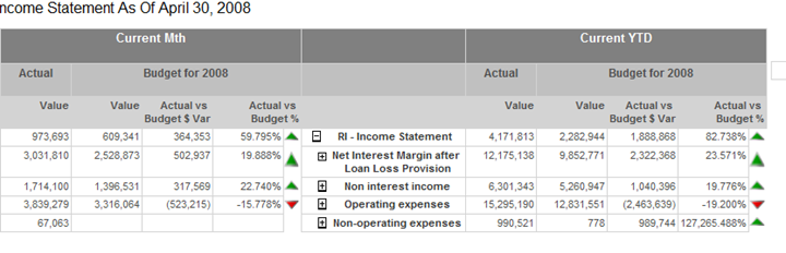
Indicators, a new feature of Reporting Services 2008 R2, let you show images for state values on your reports and avoid using custom images and expressions. Sean Boon’s recent blog shows you how to scale the indicator images. One annoying issue business users reported when working with indicators is that the indicator image stretches if the text grows and spills to the next row. For example, on the report below the second row spans two lines and its indicator images are stretched vertically.
Unfortunately, the indicator region doesn’t have a property to “fix” the image size. The only workaround for now is to enclose the entire indicator region in a rectangle: a kludgy hack especially for business users.
Visual Studio 2010 ships with updated ReportViewer controls which Brian Hartman discusses in his blog. One issue I recently run into with the Visual Studio 2008 ReportViewer ASP.NET control with a chart configured for a dynamic height (DynamicHeight property) where the chart image wouldn’t size properly. I found that the issue got fixed in the Visual Studio 2010 ReportViewer. However, in my case we weren’t ready to move to Visual Studio 2010 yet. This is what I had to do to upgrade the web application to use the Visual Studio 2010 ReportViewer control:
In web.config, replace all 9.0.0.0 version references to Report Viewer to 10.0.0.0.
Of course, if you have Visual Studio 2010, it will take of care of making the required changes for you. Finally, by upgrading to the 2010 ReportViewer as an added bonus besides fixing the dynamic height issue, you will also get the new AJAX support which eliminates page reposts and improves the end user experience.
Microsoft released the Microsoft SQL Server 2008 R2 Feature Pack. Among other things, it includes Report Builder 3.0, Reporting Services SharePoint Add-in, and PowerPivot for Excel.
https://prologika.com/wp-content/uploads/2016/01/logo.png00Prologika - Teo Lachevhttps://prologika.com/wp-content/uploads/2016/01/logo.pngPrologika - Teo Lachev2010-05-12 12:09:522016-02-17 05:18:37Microsoft SQL Server 2008 R2 Feature Pack Available
My presentation “What’s New in Reporting Services 2008 R2” for the local Atlanta.MDF group went well last night. We had some 80 people attending and I had some great questions. Too bad I couldn’t beat my previous attendance record. I guess rain and traffic were deterrent factors. Thanks for everyone who attended! I posted the presentation materials on my website. It should be available shortly on the Atlanta.MDF site as well.
There is still time to register for the online Applied Analysis Services 2008 class run on May 17th. No travel, no hotel expenses, just 100% content delivered right to your desktop! This intensive 3-day online class (14 training hours) teaches you the knowledge and skills to master Analysis Services to its fullest. Use the opportunity to ask questions and learn best practices.
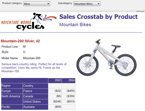
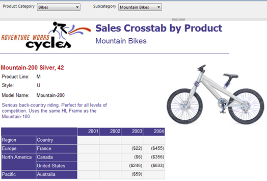
One new R2 feature that I discovered while reading the Reporting Services Recipes book, is group data synchronization. Consider the following report (download the two sample reports here):
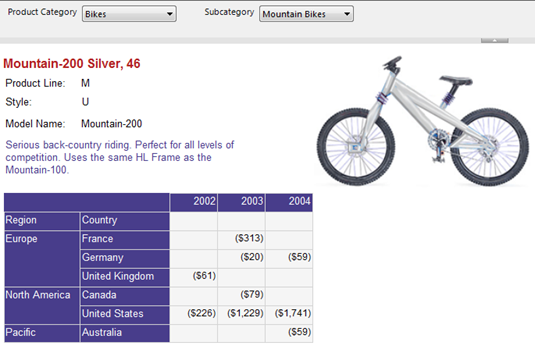
In this report, the matrix region is nested inside a list region. The list region pages (groups) on product while the nested matrx region displays the sales for the current product grouped by region and year. As you can see, Mountain-200 Sliver, 42 has data for years 2003 and 2004 but if you move to the next page, you will see that Montain-200 Silver, 46 has sales for 2002, 2003, and 2004.
What if you want to synchronize the instances of the matrix region to return the same number of columns, which in this case would it all available years in the dataset? In R2, this takes a few clicks.
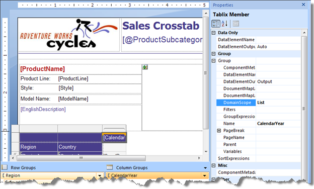
In design mode, click anywhere inside the nested matrix region so the Groups pane shows its groups.
Select the CalendarYear column group on which the matrix region pivots.
Expand the Group section in the Properties window and enter the name of the outer region in the DomainScope property. In this case, the outer region is the list region whose name is List.
Now, when you run the report, all instances of the matrix region are synchronized and have the same number of columns irrespective of the fact that they might not have data for given years.
DomainScope is similar to expression scope but not the same. DomainScope can be set on a group leaf member only. So, if the matrix region was grouping on years and quarters, you can synchronize quarters only in which case each year would show four quarters. You cannot synchronize the Year level because it’s a parent group. In addition, the domain scope can be an outer group or region. Unlike expression scopes, you cannot synchronize on a dataset.
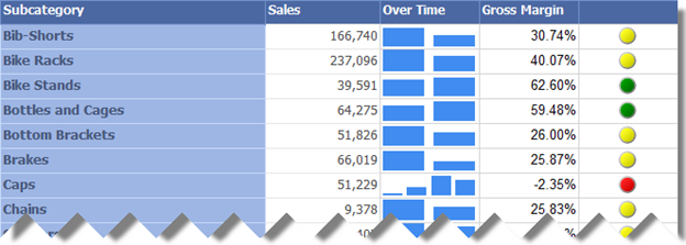
Group synchronization comes also handy when you work with sparklines. For example, the following report includes an Over Time column that shows a bar sparkline for product category sales over years.
As you can see, the Caps category has sales for four years (The AventureWorksDW2008 database has data for years 2001-2004), while Bib-Shorts category has data for two years. However, the sparklines groups are not aligned. For instance, you can’t tell which two years Bib-Shorts have sales for. To fix this:
Double-click the sparkline region to show the Chart Data window.
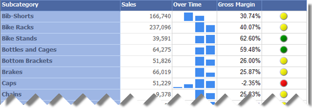
Click the CalendarYear group and set the DomainScope property to the name of the containing tablix region, Tablix1 in this case.
Now, when you run the report, you’ll see that the sparkline group ordinal position reflects the year. Thus, knowing the range of available years (2001-2004) which for clarity you can display on the report, e.g. as a subtitle, Bib-Shorts have data for years 2002 and 2003, while Bike Racks have data for 2003 and 2004.