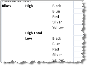
Here is a great tip thanks to Greg Galloway who pointed me to the Steve Novoselac's excellent blog. By default, Excel 2007 PivotTable stacks (hierachizes) the attributes on the report even if they are from the same dimension. For example, let's say the user wants to slice by the product hierarchy but want also some additional product attributes, such as the product color, size, etc. By default, Excel will produce the following layout:

Needless to say, this is hardly what the users want to see as they would prefer the product attributes to be displayed in a tabular format. Luckily, this is easy albeit not very intuitive.

1. Before you drop the first field on PivotTable, click the Design main menu on the ribbon (the one next to Options menu).

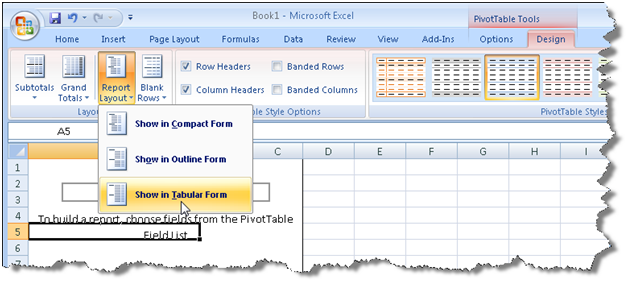
1. Expand the Report Layout drop-down menu and select Show in Tabular Form. Again, make sure that that PivotTable is empty before you do this.
2. If you want to remove subtotals, expand the Subtotals drop-down menu and select Do Not Show Subtotals.
3. Finally, to remove the +/- indicators, right-click on PviotTable and select PivotTable Options. On the Display tab, uncheck the Show Expand/Collapse Buttons.

Then, you can proceed to laying out the report as usual. Now you have a cool-looking tabular report.