Estimating Data Compression

Now that the age of in-memory databases has dawned on us, I’ve been experimenting with different aspects of VertiPaq and I find its technology fascinating. It’s safe to say that VertiPaq will propel Microsoft Business Intelligence for years to come with all of its three flavors: PowerPivot (self-service BI), Business Intelligence Semantic Model (corporate BI), and data warehousing (column-based stored indexes). Unlike Analysis Services MOLAP, which compresses data by rows, VertiPaq compresses data by columns.

Column-based compression fits business intelligence like a glove because data is typically analyzed by columns. And, the lower the data cardinality (that is the more repeating values a column has), the higher its compression rate will be. Since most columns used for analytics fit this category, you could expect 10-15 times data compression. Consequently, a half terabyte database could potentially fit into 80 GB of memory. Notice that I account for more memory because when data is brought from disk into memory, additional space is needed to accommodate index tables and other structures. So, how is this not cool? Moving to BISM, all of your data could fit into memory so you could get a head start in performance just by having a superfast storage medium!

Continuing this line of thought, I decided to take the Contoso Retail DW database and a real-life data warehouse for a spin to see how VertiPaq compresses them. I used the excellent PowerShell script that Vidas Matelis developed. Since fact tables typically contribute to 95% of the data warehouse storage space, I focused on only one fact table from both databases. To measure the VertiPaq compression, I loaded the fact tables into PowerPivot and run the script to obtain their storage space.

MOLAP

VertiPaq

Contoso (FactSales)

129 MB

35 MB

DW (20 mil fact table)

810 MB

792 MB

As you can see, the Contoso VertiPaq results are very impressive. But what happened with the real-life DW? How could VertiPaq be only marginally better than MOLAP? To analyze this further, I used the script ability to get a column compression breakdown and I’ve noticed that the following top two columns occupy the most space:

TRANS_DTLS_KEY: 400 MB (primary key)

LOG_ID: 268 MB (transaction identifier)

Both of these columns are high-cardinality columns. I used these columns in a cube drillthrough action to get the transaction details behind a cell. Subsequently, I added them to PowerPivot so I could compare the same data structures. Currently, PowerPivot doesn’t support drillthrough so adding these columns to PowerPivot is probably not needed in real life. It will be interesting to see how BISM will implement drillthrough. One thing is sure: it makes sense to leave high-cardinality attributes out of VertiPaq and possibly use report actions (if supported) to report on details.

PowerPivot Stories from the Trenches

Now that a snow blizzard has paralyzed Atlanta for a week, what a better way to start the new year than sharing a PowerPivot success story. A bank institution has approached Prologika to help them implement a solution to report the customer’s credit history so the bank can evaluate the risk for granting the customer a loan. Their high-level initial requirements call for:

  • Flexible searching and filtering to the let the bank user find a particular customer or search for the customer accounts both owned by the bank or externally reported from other banks.
  • Flexible report layout that will let the bank user change the report layout by adding or removing fields.
  • Ability to download the report locally to allow the bank user to run the report when there is no connectivity.
  • Refreshing the credit history on a schedule.

Initially, the bank was gravitating toward a home-grown solution that would require tons of custom code to implement a desktop client that uses a third-party control or ReportViewer for reporting. One cool thing about Microsoft BI and my favorite tip I share at any public event is that reduces or eliminates custom code. This may sound strange coming from someone who spent most of his career writing code but less code is indeed in the customer’s best interest. So, we suggested a solution based on PowerPivot with the following implementation highlights:

  • Implement a PowerPiivot application and import the customer and account information.
  • Allow the end user to use slicers and PivotTable filters to search and filter data.
  • Upload to PowerPivot application to SharePoint to let each bank user view and interact with the report without requiring Excel 2010 installed locally.
  • Allow the user to download the application for offline reporting. This requires Excel 2010 with PowerPivot installed locally.

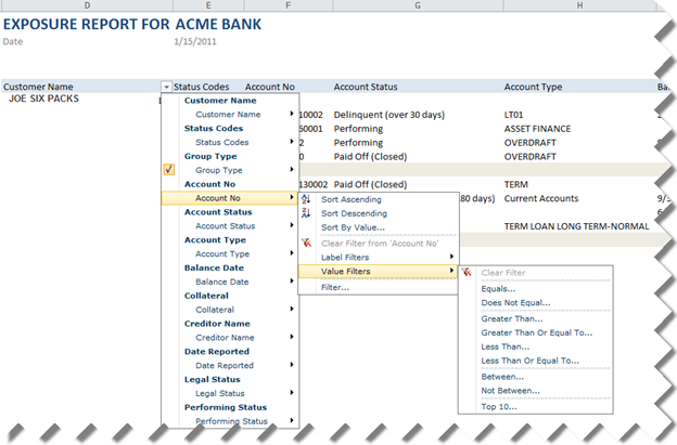
Here is a screenshot of the PowerPivot application rendered in SharePoint (sensitive information replaced to protect the innocent) that demonstrates some of the filtering capabilities that are built in Excel Services:

011511_1805_PowerPivotS1

Needless to say, this PowerPivot-based solution saved our customer a lot of time and money. True, we had to make some tradeoffs in terms of functionality and flexibility. One interesting implementation detail was that the reporting requirements required detail-level reporting at the account level instead of aggregating data. Out initial thought was that the in-memory VertiPaq database could handle this very efficiently. However, we ran into performance issues related to the fact that Excel generates MDX queries against VertiPaq and MDX is not optimized for detailed-level reporting especially when cross-joining multiple dimensions. To mitigate this issue, we took advantage of the Analysis Services Autoexists behavior that cross-joins attributes of the same dimension very efficiently. To do so, we consolidated the Customer and Account information into the Accounts table. We used the Customer table only for the Excel slicers and filtering by customer.

Looking ahead, it will be nice if a future release of PowerPivot detects that it deals with VertiPaq and generates native DAX queries instead of MDX to take a full advantage of VertiPaq. Crescent will be the first and only Microsoft client when SQL 11 ships that will generate native queries so detailed-level reporting will likely to be faster with Crescent.

PowerPivot Time Calculations

A recommended practice for implementing time calculations in PowerPivot is to have a Data table with a datetime column. Kasper de Jonge explains in more details in this blog. This approach will probably save effort when importing data from normalized schemas and won’t require specifying additional arguments to the PowerPivot time functions. However, it will undoubtedly present an issue when importing data from a star schema. A dimensional modeling best practice is to have an integer key for a Data dimension table in the format YYYYMMDD and integer foreign keys in the fact tables. Luckily, you don’t have to normalize data back to datetime when building a PowerPivot model on top of star schemas after the issue with the All filter Kasper reported a while back got fixed in PowerPivot RTM.

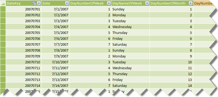
Let’s consider the AdventureWorksDW schema. Its DimDate table has an integer key (DateKey). Let’s say you import this table in PowerPivot and name it Date. This is what the resulting PowerPivot table may look like. Fact tables join the Data table on the DateKey field which is an integer key.

011511_1555_PowerPivotT1

Now you want to calculate YTD values. Since we don’t have scope assignments in PowerPivot, you need to implement a time calculation for each field that you need YTD. For the SalesAmount field, you can use the following DAX expression:

=TotalYTD(Sum([SalesAmount]), ‘Date'[Date], All(‘Date’))

The TotalYTD function is one of the PowerPivot time intelligence functions. The second argument references the Date column in the Date table which must be of datetime. Finally, the third argument overwrites the evaluation context by telling PowerPivot to evaluate the expression irrespective of date selection, that is across all dates. A nice enhancement for a future PowerPivot (aka BISM) release is to provide some sort of UI to allow the modeler to flag which column in the Data table is a datetime column in order to avoid the All flag.