In my previous blog, I talked about Hive. Hive provides a SQL-like layer on top of Hadoop so you don’t have write tons of MapReduce code to query Hadoop and to aggregate and join data. To facilitate working with Hive, Microsoft introduced a Hive ODBC driver (as of this writing, the driver is only available to Hadoop on Azure CTP subscribers). You can use this driver to connect to Hive running on Microsoft Azure or your local Hadoop server. Danny Lee has provided detailed instructions of how to do the former. I’ll show you how to use it to connect to your local Hive server.
Start the Hive Server
If you use the Cloudera VM, the Hive server is not running by default. This service allows external clients to connect to Hive. To start it:
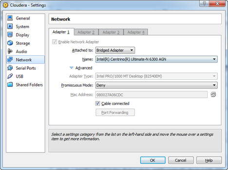
Configure your Cloudera VM to obtain an IP address on your network. To do so in Oracle Virtual Box, go to the VM settings (Network tab), and change the network adapter to Bridge Adapter.
Start the Cloudera VM and open the command prompt.
3.. If your host OS is Windows, edit the C:\Windows\System32\drivers\etc\host file and add an entry for that address, e.g.:
192.168.1.111 cloudera
4. Ping the VM from the host OS to make sure it responds on the DNS name
C:> ping cloudera
5. Start the Hive server using this command:
[cloudera@localhost ]$ hive –service hiveserver
By default, the Hive server listens on port 10000.
Analyze Data in Excel
There are two ways to bring Hive results in Excel and both options require the Hive ODBC driver:
You can use the Hive Pane to import data. This option provides a basic user interface, called a Hive Pane, which is capable of auto-generating Hive queries.
Import Hive tables directly into PowerPivot for Excel.
Using the Hive Pane
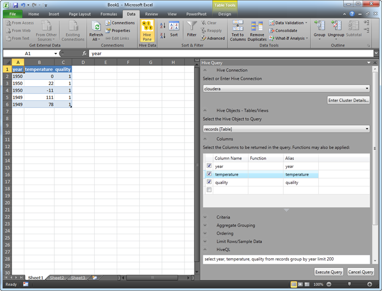
Once you install the Hive ODBC driver, you’ll get a new button in the Data ribbon group called Hive Pane.
Click the Enter Cluster Details button. In the Host field, enter whatever name you specified in the host file (cloudera in my case). Note that the default port is set to 10000. Click OK. You shouldn’t see errors at this point.
Expand the Select the Hive Object to Query and select a table. Select which columns you want to bring in. Optionally, specify criteria, aggregate grouping, and ordering. Notice that by default, the driver brings the first 200 rows but you can use the Limit Rows section to overwrite the default.
Click Execute Query to run the query and generate a table in Excel.
From there on, you can use the Excel native PivotTable and PivotChart reports to analyze data or link the data to PowerPivot.
Importing Data in PowerPivot
The second option is to bypass the Hive Pane and import a Hive table directly into PowerPivot. To do so, you need to set up a file data source first.
In Windows, go to Administrative Tools and click Data Sources (ODBC).
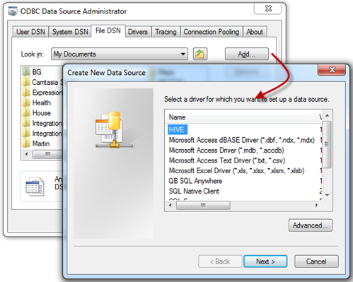
In the ODBC Data Source Administrator, click the File DSN tab, and then click the Add button.
In the Create New Data Source dialog box, select the HIVE driver.
Click Next and save the file data source, such as in the C:\Users\Teo\Documents\My Data Sources folder. Ignore the warning that pops up.
Back to the ODBC Data Source Administrator (File DSN tab), browse to the folder where you saved the file data source, select it, and click Configure. That will bring you to the same ODBC Hive Setup where you specify the Hadoop server name and port. Close the ODBC Data Source Administrator.
Back to Excel, click the PowerPivot ribbon menu, and then click the PowerPivot Window.
In the PowerPivot Window Home tab, click the From Other Sources button in the Get External Data ribbon group.
In the Table Import Wizard, select the Others (OLEDB/ODBC) option, and then click Next.
In the Specify a Connection String, click the Build button to open the Data Link Properties.
Select the Provider tab and then select the Microsoft OLE DB Provider for ODBC Drivers.
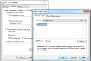
Select the Connection tab. Select the Use Connection String option, and then click the Build button.
In the Select Data Source dialog box, browse to the folder where you saved the file data source, select it, and then click OK to return back to the Data Link Properties.
The Connection String field should now be populated with the following text:
10. Click the Test Connection button to verify connectivity. Click OK to return to the Table Import Wizard which should now have the following connection string:
A long time ago, I wrote a blog about possible reasons for Reporting Services reports to time out. This issue raised its head again; this time in SharePoint 2010 environment where long running reports would time out after about 2 minutes. To resolve:
On each Web Front End (WFE) server, edit the web.config file of the SharePoint web application. For the default web application, the web.config file is located in C:\inetpub\wwwroot\wss\VirtualDirectories\80.
Find the httpRuntime element and change the executionTimeout setting. The default value is 110 seconds.
Save the web.config file. No need for iisreset since the ASP.NET process will apply the settings on change.
As a side note, you shouldn’t have such report hogs but sometimes you can’t avoid them. In this case, the end users requested a report that includes pretty much all measures in the cube sliced by the dimension with the highest cardinality so they can export it to Excel and analyze it in a pivot table.
UPDATE 6/29/2012
There is more to report timeouts if you have a SharePoint custom page that wraps the SQL Server Reporting Services ReportViewer webpart. In this case, the page won’t overwrite the timeout for the AJAX script manager control. To avoid this, make the following changes to the SharePoint master page:
1. Open the SharePoint Designer and connect to the site.
2. In the Navigation pane, click the Master Pages section.
3. Right-click the master page that site uses (v4.master is the default master page), and click Edit File in Advanced Mode.
4. Locate the ScriptManager element and add an AsyncPostBackTimeout element, as follows:
5. Save the master page, check it in, and approve it (if you use the SharePoint publishing features).
Important If the reports are deployed to a SharePoint subsite, use the SharePoint Designer to connect to the subsite and make the changes to the subsite master page.
Writing MapReduce Java jobs might be OK for simple analytical needs or distributing processing jobs but it might be challenging for more involved scenarios, such as joining two datasets. This is where Hive comes in. Hive was originally developed by the Facebook data warehousing team after they concluded that “… developers ended up spending hours (if not days) to write programs for even simple analyses”. Instead, Hive offers a SQL–like language that is capable of auto-generating the MapReduce code.
The Hive Shell
Hive introduces the notion of a “table” on top of data. It has its own shell which can be invoked by typing “hive” in the command window. The following command shows the Hive tables. I have defined two tables: records and records_ex.
[cloudera@localhost book]$ hive
hive> show tables;
OK
records
records_ex
Time taken: 4.602 seconds
hive>
Creating a Managed Table
Suppose you have a file with the following tab-delimited format:
1950 0 1
1950 22 1
1950 -11 1
1949 111 1
1949 78 1
The following Hive statement creates a records table with three columns.
hive> CREATE TABLE records (year STRING, temperature INT, quality INT)
ROW FORMAT DELIMITED
FIELDS TERMINATED BY ‘\t’;
Next, we use the LOAD DATA statement to populate the records table with data from a file located on the local file system:
LOAD DATA LOCAL INPATH ‘input/ncdc/micro-tab/sample.txt’
OVERWRITE INTO TABLE records;
This causes Hive to move the file to its repository on local file system (/hive/warehouse). Therefore, by default, Hive will manage the table. If you drop the table, Hive will delete the source data.
Creating an External Table
What if the data is already in HDFS and you don’t want to move the files? In this case, you can tell Hive that the table will be external to Hive and you’ll manage the data. Suppose that you’ve already copied the sample.txt file to HDFS:
CREATE EXTERNAL TABLE records_ex (year STRING, temperature INT, quality INT)
LOCATION ‘/user/cloudera/records_ex’;
LOAD DATA INPATH ‘/input/ncdc/sample.txt’
OVERWRITE INTO TABLE records_ex
The EXTERNAL clause causes Hive to leave the data where it is without even checking if the file exists. The INPATH clause points to the source file. The OVEWRITE clause causes the existing data to be removed.
Querying Data
The Hive SQL variant language is called HiveQL. HiveQL does not support the full SQL-92 specification as this wasn’t a design goal. The following two examples show how to select all data from our table.
hive> select * from records_ex;
OK
1950 0 1
1950 22 1
1950 -11 1
1949 111 1
1949 78 1
Time taken: 0.527 seconds
hive> SELECT year, MAX(temperature)
> FROM records
> WHERE temperature != 9999
> AND quality in (1,2)
> GROUP BY year;
Total MapReduce jobs = 1
Launching Job 1 out of 1
Number of reduce tasks not specified. Estimated from input data size: 1
In order to change the average load for a reducer (in bytes):
As you can see from the second example, Hive generates a MapReduce job. Please don’t make any conclusions from the fact that this simple query takes 26 seconds on my VM while it would take a millisecond to execute on any modern relational database. It takes quite a bit of time to instantiate MapReduce jobs and end users probably won’t query Hadoop directly anyway. Besides, the performance results will probably look completely different with hundreds of terabytes of data.
In a future blog on Hadoop, I plan to summarize my research on Hadoop and recommend usage scenarios.
https://prologika.com/wp-content/uploads/2016/01/logo.png00Prologika - Teo Lachevhttps://prologika.com/wp-content/uploads/2016/01/logo.pngPrologika - Teo Lachev2012-06-24 23:54:002018-01-15 17:35:33MS Guy Does Hadoop (Part 3 – Hive)
In part 1 of my Hadoop adventures, I walked you through the steps of setting the Cloudera virtual machine, which comes with CentOS and Hadoop preinstalled. Now, I’ll go through the steps to run a small Hadoop program for analyzing weather data. The program and the code samples can be downloaded from the source code that accompanies the book Hadoop: The Definitive Guide (3rd Edition) by Tom White. Again, the point of this exercise is to benefit Windows users who aren’t familiar with Unix but are willing to evaluate Hadoop in Unix environment.
Downloading the Source Code
Let’s start by downloading the book source and the sample dataset:
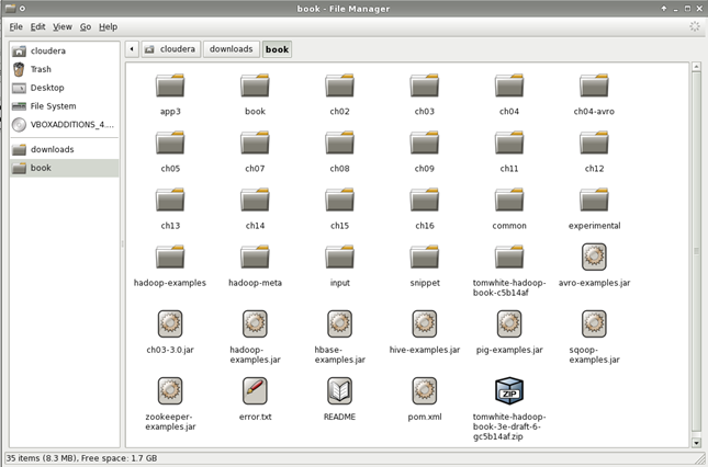
Start the Cloudera VM, log in, and open the File Manager and create a folder downloads as a subfolder of the cloudera folder (this is your home folder because you log in to CentOS as user cloudera). Then, create a folder book under the downloads folder.
Open Firefox and navigate to the book source code page, and click the Zip button. Then, save the file to the book folder.
Open the File Manager and navigate to the /cloudera/downloads folder. Right-click the book folder and click Open Terminal Here. Enter the following command to extract the file: [cloudera@localhost]$ unzip tomwhite-hadoop-book-3e-draft-6-gc5b14af.zip
Unzipping the file, creates a folder tomwhite-hadoop-book-c5b14af and extracts the files in it. To minimize the number of folder nesting, use the File Manager to navigate do the/book/tomwhite-hadoop-book-c5b14af folder, press Ctrl+A to copy all files and paste them into the /cloudera/downloads/books folder. You can then delete the tomwhite-hadoop-book-c5b14af folder.
Building the Source Code
Next, you need to compile the source code and build the Java JAR files for the book samples.
Tip I failed to build the entire source code from the first try because my virtual machine ran out of memory when building the ch15 code. Therefore, before building the source, increase the memory of the Cloudera VM to 3 GB.
Download and install Maven. Think of Maven as MSBUILD. You might find also the following instructions helpful to install Maven.
Open the Terminal window (command prompt) and create the following environment variables so you don’t have to reference directly the Hadoop version and folder where Hadoop is installed:
In the terminal window, navigate to the /cloudera/downloads/book and build the book source code with Maven using the following command. If the command is successful, it should show a summary that all projects are built successfully and place a file hadoop-examples.jar in the book folder.
Next, copy the input dataset with the weather data that Hadoop will analyze. For testing purposes, we’ll use a very small dataset which represents the weather datasets kept by National Climatic Data Center (NCDC). Our task it to parse the files in order to obtain the maximum temperature per year. The mkdir command creates a /user/cloudera/input/ncdc folder in the Hadoop file system (HDFS). Next, we copy the file from the local file system to HDFS using put.
1949 111 # the max temperature for 1949 was 11.1 Celsius
1950 22 # the max temperature for 1950 was 2.2 Celsius
Understanding the Map Job
The book provides detailed explanation of the source code. In a nutshell, the programmer has to implement:
A Map job
(Optional) a Reduce job – You don’t need a Reduce job when there is no need to merge the map results, such as when processing can be carried out entirely in parallel (see my note below).
An application that ties the Mapper and the Reducer.
Note What I learned from the book is that Hadoop is not just about analyzing data. There is nothing stopping you to write a Reduce job that does some kind of processing to take advantage of the distributed computing capabilities of Hadoop. For example, the New York Times used Amazon’s EC2 compute cloud and Hadoop to process four terabytes of scanned public articles and convert them to PDFs. For more information, read the “Self-Service, Prorated Supercomputing Fun!” article by Derek Gottfrid.
if (airTemperature != MISSING && quality.matches(“[01459]”)) {
context.write(new Text(year), new IntWritable(airTemperature));
} } }
The code simply parses the input file line by line to extract the year and temperature reading from the fixed-width input file. So, no surprises here. Imagine, you’re an ETL developer and decide to use code to parse a file instead of using the SSIS Flat File Source, which relies on a data provider to do the parsing for you. However, what’s interesting in Hadoop is that the framework is intrinsically parallel and distributes the ETL job on multiple nodes. The map function extracts the year and the air temperature and writes them to the Context object.
(1950, 0)
(1950, 22)
(1950, −11)
(1949, 111)
(1949, 78)
Next, Hadoop processes the output, sorts it and converts it into key-value pairs. In this case, the year is the key, the values are the temperature readings.
FileInputFormat.addInputPath(job, new Path(args[0]));
FileOutputFormat.setOutputPath(job, new Path(args[1]));
job.setMapperClass(MaxTemperatureMapper.class);
job.setReducerClass(MaxTemperatureReducer.class);
job.setOutputKeyClass(Text.class);
job.setOutputValueClass(IntWritable.class);
System.exit(job.waitForCompletion(true) ? 0 : 1);
} }
Summary
Although simple and unassuming, the MaxTemperature application demonstrates a few aspects of the Hadoop inner workings:
You copy the input datasets (presumably huge files) to the Hadoop distributed file system (HDFS). Hadoop shreds the files into 64 MB blocks. Then, it replicates each block three times (assuming triple replication configuration): to the node where the command is executed, and two additional nodes if you have a multi-node Hadoop cluster to provide fault tolerance. If a node fails, the file can still be assembled from the working nodes.
The programmer writes Java code to implement a map job, a reduce job, and an application that invokes them.
The Hadoop framework parallelizes and distributes the jobs to move the MapReduce computation to each node hosting a part of the input dataset. Behind the scenes, Hadoop creates a JobTracker job on the name node and TaskTracker jobs that run on the data nodes to manage the tasks and report progress back to the JobTracker job. If a task fails, the JobTracker can reschedule the job to run on a different tasktracker.
Once the map jobs are done, the sorted map outputs are received by the node where the reduce job(s) are running. The reduce job merges the sorted outputs and writes the result in an output file stored in the Hadoop file system for reliability.
Hadoop is a batch processing system. Jobs are started, processed, and their output is written to disk.
https://prologika.com/wp-content/uploads/2016/01/logo.png00Prologika - Teo Lachevhttps://prologika.com/wp-content/uploads/2016/01/logo.pngPrologika - Teo Lachev2012-06-10 00:50:002016-02-16 07:28:18MS BI Guy Does Hadoop (Part 2 – Taking Hadoop for a Spin)
With Big Data and Hadoop getting a lot of attention nowadays, I’ve decided it’s time to take a look so I am starting a log of my Hadoop adventures. I hope it’ll benefit Windows users especially BI pros. If not, at least I’ll keep a track of my experience, so I can recreate it if needed. Before I start, for an excellent introduction to Hadoop from a Microsoft perspective, watch the talk on Big Data – What is the Big Deal? by David Dewitt. Previously, I’ve experimented and I got my feed wet with Apache Hadoop-based Services for Windows Azure, which is the Microsoft implementation for Hadoop in the cloud, but I was thirsty for more and wanted to dig deeper. Microsoft is currently working on CTP of Hadoop-based Services For Windows, which will provide a supported environment for installing and running Hadoop on Windows. While waiting, O’Reilly was king enough to send me a review copy of Hadoop – The Definitive Guide, 3rd Edition, by Tom White. Since Hadoop is an open-source project, I had to rediscover and relearn something I thought I would never had to since my university days – Unix, or to be more precise its CentOS Linux variant which is installed on the Cloudera VM. So, part 1 is about setting up your environment.
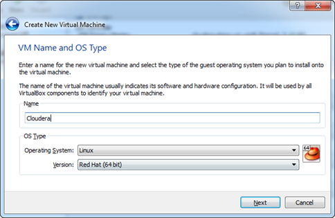
From the book, I discovered that Cloudera has a virtual machine for Virtual Box. I have VirtualBox on my Windows 7 laptop so I could run SharePoint 2010 (available in x64 only). VirtualBox is a great piece of software that was originally developed by Sun Microsystems and currently owned by Oracle. So, I’ve decided to take the VM shortcut since I don’t have much time to mess around with Cygwin, Java, etc. After downloading and double-extracting the Cloudera file, I created a new VirtualBox machine and I’ve made the following changes.
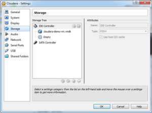
On the next step, I increased the memory to 2GB (recommended by Cloudera). In the Virtual Hard Disk step, I chose the “Use existing hard disk” option and pointed to the vmdi file I extracted from the Cloudera downloadable. Then, in the Settings page for the new VM, I’ve changed the storage to use the IDE controller instead of SATA which Cloudera said that the VM might have an issue with.
Once this was done, I was able to start the VM, which automatically logged me into CentOS as user cloudera. The first challenge I had to overcome was installing the VirtualBox Guest Editions for Linux in order to be able to resize the window and move the mouse cursor in and out without having to hold the right Ctrl key. This turned out to be more difficult than expected. The final solution took the following steps:
Once you’ve started the guest OS, in the VM menu toolbar click Install Guest Additions to mount the disk.
Open the File Manager and navigate to the /etc/yum.repos.d folder. Right-click the folder and click Open Terminal Here.
In the command window, type the following command to elevate your privileges:
$ su
Enter the password (claudera) when prompted
Open the Vi editor to edit the Cloudera-cdh3.repo as mentioned in the Cloudera VM demo note by typing this command.
su -c vi Cloudera-cdh3.repo
Change the baseurl line (changes in bold):
[Cloudera-cdh3]
name=Cloudera’s Distribution for Hadoop, Version 3
Press ESC to go to command mode and type :wq to save and exit vi.
Tip: To edit files in a more civilized way, click the File Manager icon in the menu bar at the bottom of the shell. However, you won’t have access to save files. As a workaround, launch the File Manager with elevated permissions as follows:
$ su –c Thunar
Enter the following command to install a few utilities and development kernel:
Then navigate to the media folder and run the Guest Additions file. $ cd /media
$ cd VBOXADDITIONS_4.1.16_78094
$ ./VBoxLinuxAdditions.run
This should install the guest additions successfully. If you see any error messages, execute additional packages with yum as requested.
Next, you can verify the Hadoop installation by executing the steps in the Starting Hadoop and Verifying it is Working Properly section in the Hadoop Quick Start Guide.
https://prologika.com/wp-content/uploads/2016/01/logo.png00Prologika - Teo Lachevhttps://prologika.com/wp-content/uploads/2016/01/logo.pngPrologika - Teo Lachev2012-06-04 02:45:002021-02-16 03:52:23MS BI Guy Does Hadoop (Part 1 – Getting Started)
Scenario: A SharePoint 2010 scale-out farm with two application servers:
APP1 – Runs Excel Calculation Services (ECS)
APP2 – Runs PowerPivot for SharePoint (R2 or 2010)
Do you need to start ECS on APP2 in order for PowerPivot for SharePoint to work?
Answer: You don’t but if you don’t have the updated Analysis Services OLE DB Provider on APP01, you’ll get the dreaded “Failed to create new connection…” error when you browse the PowerPivot workbook. SharePoint ships with the SQL 2008 ADO MD, MSOLAP, etc. stack; not the R2 or later components. Therefore, you must upgrade the OLE DB provider (R2 or 2010 depending on the PowerPivot version) as explained in the How to: Install the Analysis Services OLE DB Provider on an Excel Services Computer topic in Books Online.
Thanks to Dave Wickert for clarifying this.
https://prologika.com/wp-content/uploads/2016/01/logo.png00Prologika - Teo Lachevhttps://prologika.com/wp-content/uploads/2016/01/logo.pngPrologika - Teo Lachev2012-06-02 15:55:002016-02-16 07:32:22Is Excel Calculation Services Needed on a PowerPivot for SharePoint Application Server?
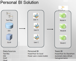
This is a blog post that I’ve been planning for a while. With the ever-increasing power of laptops and desktop computers and declining hardware prices, personal BI is on the rise. Typically, a new technology usually has a self-propelled upward spiral to a point – vendors are talking about it to clients, executives are talking about it on golf courses, consultancies are talking about it, and are rushing to fill in the void. There is a lot of money to be made with a lot of misinformation and sometimes outright lies. I’ll be quick to point out that personal BI alone is not going to fix your BI and data challenges. However, it can complement organizational BI well and open possibilities when organizational BI alone is not enough. You might find the following information interesting when you’re contemplating which way to go.
Organizational BI
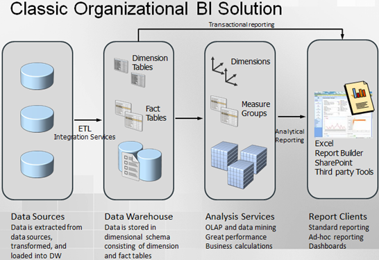
Organizational BI is a set of technologies and processes for implementing an end-to-end BI solution where the implementation effort is shifted to BI Pros. An example of a “classic” (and somewhat simplified) organizational BI solution follows.
PROS
Pervasive business intelligence – Available to all users across the enterprise, subject to security policies.
Single version of the truth with trusted data – Provides accurate and trusted analysis and reporting. Data is clean, validated, and secure.
Rich feature set –OLAP, data mining, KPIs, dashboards. For more information about using Analysis Services for organizational BI, read my blog Why an Analytical Layer?
Performance – High performance and scalability with massive data volumes
CONS
Effort – Significant development effort might be required
Skills – Specialized skills required (BI pros)
More rigid – Less flexible to react to new business requirements
PERSONAL BI
Personal BI provides business users tools for implementing ad-hoc BI models with help, guidance and supervision from IT (see below). In the Microsoft BI world, the tool for personal BI is PowerPivot with its two flavors: PowerPivot for Excel and PowerPivot for SharePoint.
PROS
Offloads effort from IT – Anyone can implement BI models if they have access to data. However, IT must still provide ongoing guidance and supervision, such as to provide access to data, to implement more advanced business calculations, to monitor the shared environment where the BI models are deployed. Therefore, I believe more in “managed” personal BI than just personal BI.
Knowledge domain expertise – Business users should know their domain better than IT.
Data mashups — Easy to mix data from different data sources.
Data exploration – Let business users explore data and tell IT what they really want before BI pros take over.
CONS
“Spreadmarts” – Proliferation of models. Which model do you trust?
Data integrity and validation issues – If users don’t import data that is already validated, such as importing data stored in the company’s data warehouse, reports probably cannot be trusted.
Power users – In reality, personal BI requires power users. In my experience, regular users don’t have the desire, skills, and time to create models. A case in point – a major organization decided to embrace a popular tool for personal BI but hired a consultancy to implement the reports! Have you heard from your users that they want operational reports, preferably delivered to them via subscriptions?
Security issues – Another burden on IT to secure data and make sure that data is not compromised when the business user imports it and share the model with another user.
So, each approach has pros and cons. Instead of exclusivity, consider using them together. For example, implement organizational BI for pervasive BI and single version of the truth, coupled with isolated scenarios for personal BI, such as when the data is not in the data warehouse or when users need to mash up data.
https://prologika.com/wp-content/uploads/2016/01/logo.png00Prologika - Teo Lachevhttps://prologika.com/wp-content/uploads/2016/01/logo.pngPrologika - Teo Lachev2012-05-27 22:22:002016-02-16 07:35:59Organizational BI vs. Personal BI
I had a presentation on the BI Semantic Layer and Tabular modeling for the Atlanta BI Group on Monday. Midway during the presentation, a DBA asked why we need an analytical layer on top of data. I’m sure that those of you who are familiar with traditional reporting and haven’t discovered yet Analysis Services might have the same question so let’s clarify.
Semantic layer
In general, semantics relates to discovering the meaning of the message behind the words. In the context of data and BI, semantics represents the user’s perspective of data: how the end user views the data to derive knowledge from it. As a modeler, your job is to translate the machine-friendly database structures and terminology into a user-friendly semantic layer that describes the business problems to be solved. To address this need, you create a semantic layer. In the world of Microsoft BI, this is the Business Intelligence Semantic Model (BISM). The first chapter (you can download it from the book page) of my latest book “Applied Microsoft SQL Server 2012 Analysis Services (Tabular Modeling)” explains this in more details.
Reducing reporting effort
Suppose that your boss comes one day and tells you that IT spends too much effort on creating operational reports. Instead, he wants to minimize cost and empower the business users to create their own reports. One of the nice features of Analysis Services is that the entity relationships become a part of the model. So, end users don’t have to know how to relate the Product to Sales entities. They just select which fields they want on the report and the model knows how to relate and aggregate data.
Performance
Analysis Services is designed to provide excellent performance when aggregating massive amounts of data. For example, in a real-life project we are able to achieve delivering operational reports within milliseconds that require aggregating a billion rows. Try to do that with relational reporting, especially when you need more involved calculations, such as YTD, QTD, parallel period, etc. Having an analytical layer might save you millions of dollars to overcome performance limitations (to a point) with relational reporting by purchasing MPP systems.
Single version of the truth
The unfortunate reality that we’re facing quite often is that many important business metrics end up being defined and redefined either in complex SQL code or reports. This presents maintenance, implementation, and testing challenges. Instead, you can encapsulate metrics where they belong – in your analytical model. As an added bonus, you will be able to use an expression language (MDX or DAX) that is specifically designed for business calculations. Moreover, the modeler can define key performance indicators (KPIs).
Additional BI possibilities
This goes hand in hand with 2, but the point that I want to emphasize here is that many reporting tools are designed to integrate and support Analysis Services well. For example, Microsoft provides Excel on the desktop and the SharePoint-based Power View tool that allows business users to create their own reports. An analytical layer opens also additional possibilities, such as performance dashboards.
Security
How much time do you spend implementing custom security frameworks for authorizing users to access data they are allowed to see on reports? Moving to Analysis Services, you’ll find that the model can apply security on connect. I wrote more about this in my article Protect UDM with Dimension Data Security.
Isolation
Because an analytical layer sits on top of the relational database, it provides a natural separation between reports and data. For example, assuming distributed deployment, a long-running ETL job in the database won’t impact the performance of the reports serviced by the analytical layer.
I’ll be presenting “The Analysis Services 2012 Tabular Model” for the Atlanta BI Group on Monday, May 21st. And, Darren Herbold will share some great insights harvested from a real-life project of how to use SSIS to integrate with Salesforce.com. I hope you can make the event, which will be sponsored by Prologika.
“SQL Server 2012 introduces the BI Semantic Model that gives BI pros two paths for implementing analytical layers: Multidimensional and Tabular. The Tabular model builds upon the xVelocity engine that was introduced in PowerPivot. Although not as feature-rich as Multidimensional, Tabular promotes rapid professional development and great out-of-box performance. This session introduces you to Tabular development and shares lessons learned. I’ll also discuss how Tabular and Multidimensional compare.”
https://prologika.com/wp-content/uploads/2016/01/logo.png00Prologika - Teo Lachevhttps://prologika.com/wp-content/uploads/2016/01/logo.pngPrologika - Teo Lachev2012-05-19 12:34:582016-02-16 07:39:16Presenting at Atlanta BI Group
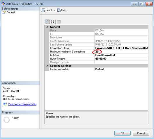
Performance tuning – my favorite! This blog originated from a quest to reduce the processing time of an SSAS cube which loads some 2.5 billion rows and includes DISCINTCT COUNT measure groups. The initial time to fully process the cube was about 50 minutes on a dedicated DELL PowerEdge R810 server, with 256 GB RAM and two physical processors (32 cores total). Both the SSAS and database servers were underutilizing the CPU resources with SSAS about 60-70 utilizations and the database server about 20-30 CPU utilization. What was the bottleneck?
By using the sys.dm_os_waiting_tasks DMV like the statement below (you can use also the SQL Server Activity Monitor), we saw a high number of CXPACKET wait types.
SELECT dm_ws.wait_duration_ms,
dm_ws.wait_type,
dm_es.status,
dm_t.TEXT,
dm_qp.query_plan,
dm_ws.session_ID,
dm_es.cpu_time,
dm_es.memory_usage,
dm_es.logical_reads,
dm_es.total_elapsed_time,
dm_es.program_name,
DB_NAME(dm_r.database_id) DatabaseName,
— Optional columns
dm_ws.blocking_session_id,
dm_r.wait_resource,
dm_es.login_name,
dm_r.command,
dm_r.last_wait_type
FROM sys.dm_os_waiting_tasks dm_ws
INNER JOIN sys.dm_exec_requests dm_r ON dm_ws.session_id = dm_r.session_id
INNER JOIN sys.dm_exec_sessions dm_es ON dm_es.session_id = dm_r.session_id
The typical advice given to address CXPACKET waits is to decrease the SQL parallelism by using the MAXDOP setting. This might help in some isolated scenarios, such as UPDATE or DELETE queries. However, the SQL Sentry Plan Explorer showed that each processing query is highly parallelized to utilize all cores. Notice in the screenshot below, that thread 16 fetches only 14,803 rows.
Therefore, the CXPACKET waits were simply caused by faster threads waiting for other threads to finish. In other words, CXPACKET wait is just a coordination mechanism between the threads being parallelized. To confirm this, we set the SQL Server MAXDOP setting to 1. Surely, the CXPACKET waits disappeared but the overall cube processing time went up as well. In our case, the biggest benefit was realized not by decreasing the SQL Server parallelism but by increasing it, by increasing the maximum number of database connections. This resulted in decreasing the overall processing time some 20%.
You need to be careful here though. While increasing the connections to max out the CPU on the SSAS server will yield the biggest gain, it might also slow down other processing, such as reports that query the cube while the database is being processed. So, as a rule of thumb, target no more than 80% CPU utilization to leave room for other tasks.