Power BI (Part 1 – Getting Started)

Microsoft BI has been criticized about its complexity and price because it requires SharePoint Server Enterprise for deploying Power Pivot models and dashboards. Microsoft introduced Office 365 (E3 or E4 plan required) and SharePoint Online (Plan 2 required) to mitigate such concerns and allow you to host Power Pivot and Power View in the cloud. Power BI is the next step in the Microsoft BI cloud strategy. As I explained in a previous blog and in the SQL Server Team blog, Power BI is essentially a cloud combo of all the self-service “power” tools (Power Pivot, Power View, Power Query, and Power Map) available on a subscription basis and running on Microsoft Azure, precluding SharePoint on-premises installation and licensing.

Microsoft has started inviting participants subscribed to the Power BI for Office 365 Preview to test the prerelease version of Power BI. During the Worldwide Partner Conference, Amir Netz, a Technical Fellow at Microsoft, demonstrated some of the Power BI most exciting features. With the exception of Power View HTML5 preview, none of these features (on-premise data refresh, natural query, and InfoNavigator) are in the Preview yet. However, Microsoft is planning to refresh the Preview on a monthly basis and push these features as they become available. Pricing hasn’t been announced yet. One disappointing news for me is that for now Microsoft doesn’t plan to support the “mixed” scenario by connecting Power View to an on-premises semantic model (Multidimensional or Tabular). In other words, in its first release Power BI will be limited to supporting Power Pivot models only, excluding organizational BI capabilities both on cloud and on premises.

The setup experience is simple and it should be familiar to you if you’ve provisioned Office 365 in the past. The invitation letter includes links to the following resources to get you started with Power BI.

  1.   View the Power BI Provisioning Video and the provisioning guide
  2.   Visit the getting started page and check out the Power BI user guide and samples
  3.   Download the Power Query and Power Map add-ins for Excel
  4.   Download the Power BI mobile app for your Windows tablet
  5.   Monitor new feature announcements on the Power BI Blog
  6.   Give us feedback on the Power BI forum

One provisioning step that you need to pay attention to is that you have to go to Users and Group section of the portal and assign yourself licenses to get access to the SharePoint sites.

083113_1355_PowerBIPart1

Once you’ve done this and navigate to the Sites and then Team Site, you’ll see a link to the Power BI site. The Power BI site supersedes Power Gallery. It’s the hosting site for deploying Power Pivot models for up to 250 MB in size.
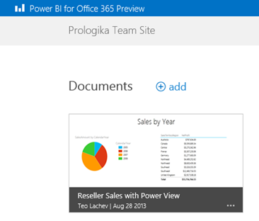
083113_1355_PowerBIPart2

Once you click deploy an Excel file with your Power Pivot model and reports, you can click it to render the reports in the browser. If the file includes a Power View report, Power BI would render it by default in Silverlight but gives you an option to try the new HTML5 preview by clicking the Try the Preview button in the bottom right corner, as explained in this blog. I ran into several issues during testing, including:

  • The Power BI site doesn’t always render
  • The Power View Field List doesn’t always show
  • The HTML5 preview generates empty rows. A list of the HTML5 supported features can be found here.

I believe that many organizations and ISVs will find Power BI attractive for cloud deployments of self-service and team BI solutions. Power BI mitigates concerns about on-premises SharePoint licensing, complexity, hardware and software overhead.

DQS Error after CU Upgrade

I installed SQL Server 2012 SP1 CU5 and I got greeted with the following error while opening Data Quality Services

082913_2223_DQSErroraft1

DqsInstaller.exe can be found by default in the C:\Program Files\Microsoft SQL Server\MSSQL11.MSSQLSERVER\MSSQL\Binn folder. However, running the dqsinstaller-upgrade didn’t fix the issue. To fix it, I had to recompile the .NET assemblies by running dqsinstaller-UpgradeDlls. BTW, CU4 is still marked as in research by the DQS team and CU5 is not even on the list.

Does Self-service BI Make Sense?

Besides data messiness (in direct proportion with the company size), another common data-related challenge that every organization nowadays is trying to tackle is how applicable self-service BI is to their business and to what extent it should be used. The tools are here and they are readily available. For example, given that Power Pivot is now natively integrated with Excel 2013, your power users will find a way to get inspired even if you don’t roll out a formal self-service BI strategy.

When self-service BI make sense

Having consulted with and trained many organizations ranging from small companies to Fortune 100 behemoths, I think that the following two scenarios appears as good reasons for self-service BI:

  1. Organizational BI is not an option. For example, a small company might not have resources to roll out an organizational BI solution, such as a management dashboard, and the data doesn’t require extensive transformation. Or, the IT department in a larger organization might be unable to keep up with business requirements, thus leaving business users on their own.
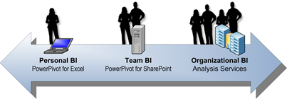
  2. Foster lateral (sometimes called divergent) thinking to generate and test ideas. Your business users might have “sketches” of alternative business scenarios or hypotheses that need to be tested quickly. For example, a business analysis in an oil services company wanted to know if the number of deployed rigs is correlated to the company’s revenue. In such cases, self-service BI can help that user to quickly mash up the revenue numbers stored in the data warehouse with the rig counts given to him as an Excel spreadsheet. Once the data that support such ideas is available and related to the organizational data, business analysts can test and converge such ideas to isolate the ones that are truly useful. Ideally, the next steps will be import the supporting data to the data warehouse so it’s available across the entire organization. Among the BI vendors, Microsoft is unique in providing the tools to implement this continuum, which might consists of self-service, team, and organizational BI steps.082913_1445_DoesSelfser1

When self-service BI doesn’t make sense

Let’s now mention scenarios when self-service BI might not be a good fit:

  1. Replacing organizational BI. By now, we all know that vendor claims stating that you don’t need organizational BI didn’t stand the test of time. Self-service BI alone is not going to solve your data integration and BI challenges. Most organizations will greatly benefit from a centralized data repository with clean and trusted data, which is typically referred to as a data mart or data warehouse, and a semantic model on top of it. Moreover, no matter how simple the tools are, self-service BI typically exceeds the skills of most information workers. Have you tried teaching a typical sales person how to create an Excel pivot report? Therefore, self-service BI should be viewed as completing, not competing, to organizational BI.
  2. Creating “spreadmarts” and Excel data dumps. If you’ve spent so much effort to centralize the data in a data warehouse, does it make sense to pull it out in different directions? If all the end users need is Excel data dumps, does it make sense to allow them to import millions of rows (probably requiring hardware and software upgrade) while a Power View on top of analytical model might be a better option? How secure that data will be on the user laptop? Finally, do you trust that the models your business users create can be used for deriving important decisions?

Still struggle with a self-service BI strategy or how to implement it? My Applied Power Pivot class and book should be able to help.

Speaking at SQL Server Innovators Guild

I’ll be speaking at the SQL Server Innovators Guild group in Greenville, SC on September 3rd. If you happen to be in the area, please join us to learn best practices for implementing an enterprise BI solution. Please confirm attendance at https://ssig201309.eventbrite.com/


Semantic Layer Flavors

Semantics relates to discovering the meaning of the message behind the words. In the context of data and BI, semantics represents the user’s perspective of data: how the end user views the data to derive knowledge from it. As a modeler, your job is to translate the machine-friendly database structures and terminology into a user-friendly semantic layer that describes the business problems to be solved and centralizes business calculations. Different vendors have different ideology and implementations of semantic layers. Some, such as Oracle and MicroStrategy, implement the semantic layer as a thin, pass-through layer whose main goal is to centralize access to data sources, metadata and business calculations in a single place.

A Fortune 100 company that had a major investment in Oracle engaged us to recommend a solution for complementing their OBIEE semantic layer with user-friendly reporting tool that would allow end users to create ad hoc transactional reports from their Oracle Exadata-based enterprise data warehouse. In the OBIEE world, the role of the semantic layer is fulfilled by the Common Enterprise Information Model that encompasses data sources, metrics, calculations, definitions, and hierarchies. When users submit report queries, the Oracle BI Server compiles incoming requests and auto-generates native queries against the data sources plugged in the Common Enterprise Information Model.

In theory, this “thin” implementation should work pretty well. In reality, several issues surface:

  1. Performance – Any tool, either a reporting tool or semantic layer, that auto-generates queries should be highly suspect of performance issues. First, no matter how well the tool is designed, it’s unlikely that it would generate efficient queries in all cases. Second, because the tool sends the query to the underlying data source, the overall report performance is determined by how fast the data source crunches data. In this case, the organization was facing performance issues with data aggregation. To circumvent them, their BI developers have implemented summarized fact tables. Once the user reaches the lowest level of the summary fact table, OBIEE would allow the user to drill down to a chained table, such as the actual fact table. Needless to say, business users were complaining that analysis was limited to the dimensionality of the summarized fact table. Further, to avoid severe performance issues with historical reports, the BI developers have taken the “no big aggregations, no problem” approach by forcing a time filter on each request that touches the large fact tables. This effectively precluded historical analysis by year, quarter, etc.
  2. Scalability – When a query involves multiple data source, OBIEE would send a query to each data source, load the data in memory, and then join the datasets together to find matching data. This also presents performance and scalability challenges. To solve performance and scalability issues with “thin” semantic layers and biggish data, organizations ultimately resort to expensive back-end MPP systems, such as Teradata or Netezza, which can parallelize data crunching and compensate for inefficient auto-generated queries.
  3. Common Denominator – You’re limited you to a subset of supported features of the underlying data source.
  4. Vendor Dependency – Such an architecture ultimately locks you in the data sources supported by the vendor. What happens when there is a new version of the data source that has some cool new features? Well, you need to wait until the vendor officially supports the new version and its extensions.

In the Microsoft BI world, the role of the semantic layer is fulfilled by the Business Intelligence Semantic Model (BISM). BISM is an umbrella name that encompasses two technologies: Multidimensional for implementing OLAP cubes and Tabular for designing relational-like models. The big difference is that by default both Multidimensional and Tabular store data on the server. In order words, from a data perspective, you can view BISM and its default storage mode (MOLAP for Multidimensional and xVelocity for Tabular) as a disk-based (MOLAP) or in-memory (xVelocity) cache of the data in your data warehouse. This proprietary storage is designed for fast data crunching even with billions of rows. You pay a price for loading and refreshing the data but you enjoy great query performance with historical and trend reports. And, you get a great ROI because you may not need an expensive MPP appliance or excessive data maintenance. When sent to BISM, queries are served by BISM, and not by the RDBMS. No need for summarized tables and time filters.

DAX Variance Calculations

Variance calculations are a common BI requirement but good reference material is lacking. How do we create them in DAX? Let’s say you need to calculate the variance between this month sales and the previous month sales.

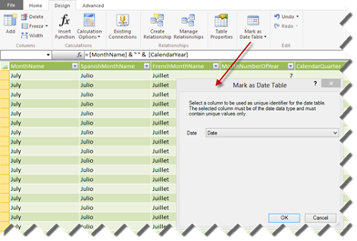
  1. DAX date functions require a Date table. They won’t work if you don’t have a separate Date table. They also require that you tell PowerPivot (or Tabular) about your Date table. So, as a first step select the Date table, go to the Design ribbon, and then click Mark as Date Table. PowerPivot will infer the column of the date data type (you must have such a column).

081513_1449_DAXVariance1

  1. Sort the Month column with custom sort. For example, if your Month column returns the month in MMM-YY format, sort that column by another integer column in the format YYYYMM. More on this in a moment.
  2. Define a new calculated measure using the following formula:

=SUM(ResellerSales[SalesAmount]) – CALCULATE(SUM(ResellerSales[SalesAmount]), PREVIOUSMONTH(‘Date'[Date]))

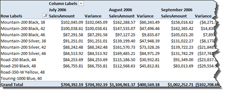
What’s going on here? The formula needs to work irrespective of the month on the report. In other words, if we put months on columns, each month will act as of that month. That’s why we need a calculated measure. The first SUM returns the aggregated sales for the month. The CALCULATE function is used to overwrite the context because we want to get to the last month sales. To do this, we pass the PREVIOUSMONTH function as a second argument and point it to use the Date column in the Date table as we do with other DAX date-related functions.

081513_1449_DAXVariance2

Here is something important. This report won’t work with just months on columns if your Month column returns the name of the month only. That’s because the month name will be repeating across years. This is why the PREVIOUSMONTH documentation insists on having both year and month on the report.

“To see how this works, create a PivotTable and add the fields, CalendarYear and MonthNumberOfYear, to the Row Labels area of the PivotTable.”

If you don’t want to add the year to reports, add a MonthName calculated column to your Date table with the following formula: = [MonthName] & ” ” & [CalendarYear] that makes the month unique across years and another column MonthNameSort to sort by with the following formula: =[CalendarYear] * 100 + [MonthNumberOfYear]. Then sort the first column by the second. To do this, in the PowerPivot window, click any cell in the MonthName column. Then, in the Home ribbon, click the Sort by Column button and choose the MonthNameSort as the sort by column. Use the MonthName column on the report, as I’ve done in the screenshot above.

Further considerations:

  1. If you want to calculate a variance between parallel periods, use the DAX ParallelPeriod() function.
  2. While a clumsy way exists in PowerPivot Tabular to handle multiple relative dates (see the “Calculating many time periods within a single measure formula” section in the DAX Samples white paper), the formulas must still reference a specific measure, e.g. SalesAmount. That’s because Tabular doesn’t currently support scope assignments that allow you to create generic “shell dimensions” spanning multiple measures.
  3. What if you want the variance to work across months, quarters, and years? Because Tabular doesn’t support functions for hierarchy navigation and no PreviusPeriod() function exists, you have to resort to the DAX Samples workaround to adjust the formulas depending on what level you are in the Date hierarchy, such as to use PreviousMonth() if you are at the month level and PreviousYear() if you are at the year level.

Refreshing Excel File in PowerPivot from SharePoint

A couple of SharePoint-related questions from students taking my PowerPivot class that are worth sharing.

Question: Can I import data from and auto-refresh an Excel file deployed to a SharePoint library in PowerPivot?

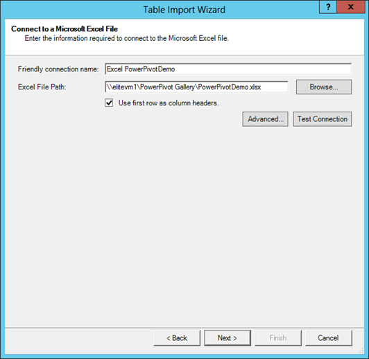
Answer: Yes, if you use WebDAV and specify the UNC path to the file. WebDAV requires the Windows Server Desktop Experience feature to be installed and the WebClient service to be started:

081013_1851_RefreshingE1

Question: If major and minor (draft) versioning is enabled in the PowerPivot Gallery, is there a way to configure PowerPivot to create major versions only on refresh instead of minor versions?

Answer: This is not supported natively by PowerPivot because the snapshot process is not configurable. A possible workaround is to configure a SharePoint workflow to promote minor versions to major versions. As a side note, you should be careful with maintaining version history because the SharePoint content database will quickly grow. If you haven’t done so, consider configuring SharePoint to retain a limited number of versions.

Analysis Services Relationship Limitations and Workarounds

Relationships in analytical models (Multidimensional and Tabular) are both a blessing and a curse. Once defined by the modeler, relationships power “slicing and dicing” data. The analytical tool doesn’t have to worry about and include the relationships in the query because they are defined in the model and the server “knows” how to use them to aggregate the data. On the other hand, as they stand, all analytical model flavors (Multidimensional, Tabular, and PowerPivot) have inherent limitations. The following table compares relationship limitations between Multidimensional and Tabular (PowerPivot).

MultidimensionalTabular and PowerPivot
Many-to-ManySupportedNot supported
Parent-childSupportedRequires flattening the hierarchy
Role-playingSupportedNot supported
Multi-grainSupportedNot supported
Fact-to-factNot supportedSupported but rarely useful


Let’s discuss these limitations in more details.

Many-to-Many

The classic example of a many-to-many relationship is a joint bank account that is owned by multiple customers. Many-to-many relationships are natively supported in Multidimensional and the server produces correct results when aggregating the data. Tabular and PowerPivot don’t support many-to-many out of the box. When the relationship One-To-Many flow is reversed through a bridge table, Tabular will let you continue but produce wrong results. In PowerPivot, this limitation manifests with the “Relationships might be needed” warning in the PowerPivot Field List. The workaround is to introduce DAX explicit measures for each column that requires aggregation using the formula =CALCULATE (SUM (FactTable[Column] ), BridgeTable). On the upside, due to the Tabular memory-resident nature, expect M2M over a large fact table to perform much better in comparison with Multidimensional.

Parent-Child

A parent-child relationship defines a recursive join between two columns, such as an employee and a manager. This relationship type is supported natively in Multidimensional but requires flattening the hierarchy using DAX calculated columns for each level in the hierarchy. Flattening the hierarchy is accomplished by using DAX PATH-related functions.

Role-playing

A role-playing relationship allows a dimension (lookup) table to be joined multiple times to a fact table, such as to join a Date dimension multiple times to a Sales fact table in order to support aggregating the fact data by OrderDate, ShipDate, and DueDate. Multidimensional supports role-playing relationships natively. Tabular doesn’t and flags only one of the relationships as active. The first (and recommended for most scenarios) workaround is simply to reimport the Date table as many times as needed. This gives you the flexibility to control the schema and data between the Date table instances, e.g. the ShipDate table includes only valid ship dates, at the expense of storage and increased model complexity. The second more complicated workaround is to create calculated measures, such as ShipAmount, DueAmount, etc., that use the DAX USERELATIONSHIP function to traverse the inactive relationships. This approach presents maintenance challenges because the chances are that the fact table will have many columns and you’ll have to create role-playing variants for each measure that needs to be aggregated.

Multi-grain

A multi-grain relationship exists when a dimension joins a fact table at a higher level than the dimension key. For example, you might have an Organization table that goes all the way down to business unit. However, an Expenses fact table might record expenses at a higher level in the organizational hierarchy, such as Division. Consequently, the modeler needs to set up a relationship from the Expenses fact table to the Division column as opposed to the Business Unit column (dimension key). Multidimensional supports this scenario out of the box. Tabular doesn’t because the joined column on the One side of the relationship must be the dimension key which uniquely identifies each row in the dimension table. The workaround is to break the Organization dimension table into two tables: Organization and OrganizationDivision in order to join the OrganizationDivision table to the Expense fact table on the Division column which is now the key column. Then, you need to join the OrganizationDivision table to the Organization table for consolidated reporting purposes, such as to see Sales and Expenses side by side.

Fact-to-fact

Suppose that your model has two fact tables: OrderHeaders and OrderLineItems. You would like to have a transactional report that shows the line items for each order. Let’s say that that the OrderHeaders fact table has an OrderID column and the OrderLineItems have a matching OrderID column. On a first thought, you might attempt to solve the problem by creating a relationship between the OrderHeaders and OrderLineItems tables. However, Multidimensional doesn’t support fact-to-fact relationships. That’s because the classic OLAP model insists on having relationships between dimensions and fact tables only. To solve this predicament in Multidimensional you need a PO Order dimension that joins both OrderHeaders and OrderLineItems tables. However, the chances are that you might end up with another complication if you take this route. This might not be applicable to the order header-line items scenario but what if the rows in the two fact tables have different dates. If a Date dimension joins them and you attempt to slice by date, the business question will be “Show me orders and order line items that have matching dates”. This might or might not be correct depending on your situation. So, this is where you’ll find that although very useful, relationship in analytical models might not be that flexible for ad hoc analysis.


Thanks to its more relaxed schema requirements, Tabular doesn’t care about the table type (dimension or fact) and it will let you set up a relationship between OrderHeaders and OrderLineItems as long as they comply to the One-To-Many rule . However, you’ll face another limitation that Tabular doesn’t support closed-loop relationships. More than likely, the OrderHeaders and OrderLineItems will have relationships to other lookup tables already, such as Account, Organization, etc. Once you create a fact-to-fact relationship, you’ll close the relationship loop. Tabular and PowerPivot will detect this and automatically deactivate the fact-to-fact relationship (its line will be dotted in the diagram view). Consequently, you must resort to the Multidimensional workaround to create an OrderHeader lookup table. Another workaround is to merge the OrderHeaders and OrderLineItems tables into a single table. Or, create a model that has only the OrderHeaders and OrderLineItems tables so you can create the fact-to-fact relationship.


Relationships are a challenging concept to grasp. As a modeler, you need to understand their limitations and workarounds while hoping that a future version of Analysis Services will relax or remove some of the existing constraints.

Performance Tuning of Tabular Models in SQL Server 2012 Analysis Services

A really impressive white paper/book with insights about Tabular performance and inner-workings. Kudos to the authors for producing this colossal resource.

“Tabular models hosted in SQL Server 2012 Analysis Service provide a comparatively lightweight, easy to build and deploy solution for business intelligence. However, as you increase the data load, add more users, or run complex queries, you need to have a strategy for maintaining and tuning performance. This paper describes strategies and specific techniques for getting the best performance from your tabular models, including processing and partitioning strategies, DAX query tuning, and server tuning for specific workloads.”