Posts

Formatting Calculated Members

Consider the following calculated member definition added to the script in an Analysis Services cube:

CREATE
MEMBER
CURRENTCUBE.[Measures].[Revenue TTM] AS ([Measures].[Revenue Amount USD], [Relative Date].[TTM]), FORMAT_STRING = “Currency”, VISIBLE = 1;

When you browse the member in Excel, you’ll find that the member is not formatted as currency. However, when you use SSMS and query the member, when you double-click the member cell in the query results, you’ll see that the value is formatted as expected. Clearly, Excel has an issue with formatting calculated members and there is a connect bug report that has been quietly sitting in the Excel bucket for years. To Microsoft credit, we have a KB article “Description of the LANGUAGE cell property in SQL Server 2005 Analysis Services”.

“However, SQL Server 2005 Analysis Services cannot determine the value of the LANGUAGE cell property or of the currency symbol for calculated members from the query context. You must specify the LANGUAGE cell property if you want to obtain a nondefault currency symbol. If you do not specify the LANGUAGE cell property, the numeric value of the cell value and the currency symbol of the cell value may not match.”

I think what they meant was specifying the Language property in the calculated member definition. Indeed, the following change causes Excel to show the calculated member formatted as currency (USD in this case):

CREATE
MEMBER
CURRENTCUBE.[Measures].[Revenue TTM] AS ([Measures].[Revenue Amount USD], [Relative Date].[TTM]), FORMAT_STRING = “Currency”, VISIBLE = 1, LANGUAGE=1033;

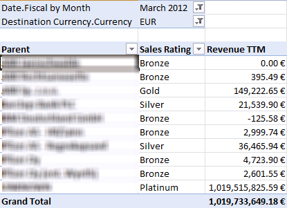
What about dynamic formatting based on the selected currency? Assuming that you have a Destination Currency dimension and includes a Locale column with the integer locale identifier, e.g. 1033 for USD, 1031 for EUR, and so on), the following script overwrites the member language and the value will be formatted based on the destination currency selected by the user:

Scope (

    [Destination Currency].[Currency].[Currency].Members,

    {

        [Measures].[Revenue TTM]

    }

    );

    Language( this ) = [Destination Currency].[Currency].Properties( “Locale” );

End
Scope;
070212_1332_FormattingC1

TIP On the subject of formatting, you might need to “pin” a calculated member to a particular currency format to avoid the OLAP browser changing the format. As a fist attempt, you might try hardcoding the currency sign, such as “$0,0.00′”. Unfortunately, Excel will ignore it and overwrite it based on the regional settings. For example, a UK user will still see “£100.00”. Hrvoje Piasevoli suggested escaping the currency symbol to prevent this from happening, e.g. create member currentcube.measures.test as 1000.01, format_string=”\$0,0.00″, language=1033;

Since I live in the USA, I have to admit I’m somewhat shielded from the localization complexities surrounding currency and date formatting. Chris Webb wrote a blog “Currency formats: should they be tied to language?” a while back that you should check as well.

Why an Analytical Layer?

I had a presentation on the BI Semantic Layer and Tabular modeling for the Atlanta BI Group on Monday. Midway during the presentation, a DBA asked why we need an analytical layer on top of data. I’m sure that those of you who are familiar with traditional reporting and haven’t discovered yet Analysis Services might have the same question so let’s clarify.

  1. Semantic layer

    In general, semantics relates to discovering the meaning of the message behind the words. In the context of data and BI, semantics represents the user’s perspective of data: how the end user views the data to derive knowledge from it. As a modeler, your job is to translate the machine-friendly database structures and terminology into a user-friendly semantic layer that describes the business problems to be solved. To address this need, you create a semantic layer. In the world of Microsoft BI, this is the Business Intelligence Semantic Model (BISM). The first chapter (you can download it from the book page) of my latest book “Applied Microsoft SQL Server 2012 Analysis Services (Tabular Modeling)” explains this in more details.

  2. Reducing reporting effort

    Suppose that your boss comes one day and tells you that IT spends too much effort on creating operational reports. Instead, he wants to minimize cost and empower the business users to create their own reports. One of the nice features of Analysis Services is that the entity relationships become a part of the model. So, end users don’t have to know how to relate the Product to Sales entities. They just select which fields they want on the report and the model knows how to relate and aggregate data.

  3. Performance

    Analysis Services is designed to provide excellent performance when aggregating massive amounts of data. For example, in a real-life project we are able to achieve delivering operational reports within milliseconds that require aggregating a billion rows. Try to do that with relational reporting, especially when you need more involved calculations, such as YTD, QTD, parallel period, etc. Having an analytical layer might save you millions of dollars to overcome performance limitations (to a point) with relational reporting by purchasing MPP systems.

  4. Single version of the truth

    The unfortunate reality that we’re facing quite often is that many important business metrics end up being defined and redefined either in complex SQL code or reports. This presents maintenance, implementation, and testing challenges. Instead, you can encapsulate metrics where they belong – in your analytical model. As an added bonus, you will be able to use an expression language (MDX or DAX) that is specifically designed for business calculations. Moreover, the modeler can define key performance indicators (KPIs).

  5. Additional BI possibilities

    This goes hand in hand with 2, but the point that I want to emphasize here is that many reporting tools are designed to integrate and support Analysis Services well. For example, Microsoft provides Excel on the desktop and the SharePoint-based Power View tool that allows business users to create their own reports. An analytical layer opens also additional possibilities, such as performance dashboards.

  6. Security

    How much time do you spend implementing custom security frameworks for authorizing users to access data they are allowed to see on reports? Moving to Analysis Services, you’ll find that the model can apply security on connect. I wrote more about this in my article Protect UDM with Dimension Data Security.

  7. Isolation

Because an analytical layer sits on top of the relational database, it provides a natural separation between reports and data. For example, assuming distributed deployment, a long-running ETL job in the database won’t impact the performance of the reports serviced by the analytical layer.

Analysis Services Processing and CXPACKET Waits

Performance tuning – my favorite! This blog originated from a quest to reduce the processing time of an SSAS cube which loads some 2.5 billion rows and includes DISCINTCT COUNT measure groups. The initial time to fully process the cube was about 50 minutes on a dedicated DELL PowerEdge R810 server, with 256 GB RAM and two physical processors (32 cores total). Both the SSAS and database servers were underutilizing the CPU resources with SSAS about 60-70 utilizations and the database server about 20-30 CPU utilization. What was the bottleneck?

By using the sys.dm_os_waiting_tasks DMV like the statement below (you can use also the SQL Server Activity Monitor), we saw a high number of CXPACKET wait types.

SELECT
dm_ws.wait_duration_ms,

dm_ws.wait_type,

dm_es.status,

dm_t.TEXT,

dm_qp.query_plan,

dm_ws.session_ID,

dm_es.cpu_time,

dm_es.memory_usage,

dm_es.logical_reads,

dm_es.total_elapsed_time,

dm_es.program_name,

DB_NAME(dm_r.database_id) DatabaseName,

— Optional columns

dm_ws.blocking_session_id,

dm_r.wait_resource,

dm_es.login_name,

dm_r.command,

dm_r.last_wait_type

FROM
sys.dm_os_waiting_tasks
dm_ws

INNER
JOIN
sys.dm_exec_requests
dm_r
ON
dm_ws.session_id = dm_r.session_id

INNER
JOIN
sys.dm_exec_sessions
dm_es
ON
dm_es.session_id = dm_r.session_id

CROSS
APPLY
sys.dm_exec_sql_text
(dm_r.sql_handle)
dm_t

CROSS
APPLY
sys.dm_exec_query_plan
(dm_r.plan_handle) dm_qp

WHERE
dm_es.is_user_process = 1

The typical advice given to address CXPACKET waits is to decrease the SQL parallelism by using the MAXDOP setting. This might help in some isolated scenarios, such as UPDATE or DELETE queries. However, the SQL Sentry Plan Explorer showed that each processing query is highly parallelized to utilize all cores. Notice in the screenshot below, that thread 16 fetches only 14,803 rows.

051512_0211_AnalysisSer1

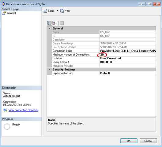
Therefore, the CXPACKET waits were simply caused by faster threads waiting for other threads to finish. In other words, CXPACKET wait is just a coordination mechanism between the threads being parallelized. To confirm this, we set the SQL Server MAXDOP setting to 1. Surely, the CXPACKET waits disappeared but the overall cube processing time went up as well. In our case, the biggest benefit was realized not by decreasing the SQL Server parallelism but by increasing it, by increasing the maximum number of database connections. This resulted in decreasing the overall processing time some 20%.

051512_0211_AnalysisSer2

You need to be careful here though. While increasing the connections to max out the CPU on the SSAS server will yield the biggest gain, it might also slow down other processing, such as reports that query the cube while the database is being processed. So, as a rule of thumb, target no more than 80% CPU utilization to leave room for other tasks.

Reducing Analysis Services Index Processing Time

Scenario: Processing a 100 GB SSAS 2012 cube on a dedicated DELL PowerEdge server (128 GB RAM with 32 logical cores) reveals that 50% of the time is spent on processing the cube indexes and building aggregations with only 20% average CPU utilization and not even a small dent to the memory consumption. It was clear that SSAS doesn’t utilize the server resources and additional tuning is required to increase the parallelism of this phase.

Solution: Following Greg Galloway’s advice, we’ve changed the OLAP\Process\AggregationMemoryLimitMin to 2 and OLAP\Process\AggregationMemoryLimitMin to 3 to increase the parallelism of the index processing. This led to 25% reduction of the overall processing time and increased the CPU utilization to 70-80%. As to how we derived to these numbers, James Rogers has a great write-up. For the sake of preserving the precious formulas:

AggregationMemoryLimitMax=Ceiling(100/(<number processing cores>-2))

AggregationMemoryLimitMin=Ceiling(100/((<number processing cores>-2)*1.5))

In case you’re curious about what these setting do, the amount of memory needed to build an aggregation is unknown up front. The engine has to estimate it based of certain factors (estimated rows, granularity attributes, measures, etc.) – and it uses the AggregationMemoryLimitMin value to ensure that if it’s estimate is wrong, that at least there will be a sufficient buffer for underestimation. Similarly, if the estimate is wrong in the upward direction, it will use the AggregationMemoryLimitMax value to trim the max value downward.

Subscription and Alerts Issues with Analysis Services in SQL Server 2012

As you probably now, Reporting Services doesn’t allow you to create subscriptions with data sources that use Windows security because subsbscriptions are run in unattended mode. Moving to SQL Server 2012, we’ll add Data Alerts to the list. This presents an issue if you use Analysis Services which only supports Windows security. The only option is to use Stored Credentials with the “Use as Windows credentials” checkbox checked. You won’t able to pass the user identity by checking “Set execution context to this account”. As with previous releases, “Set execution context to this account” works with the SQL Server data but it doesn’t work with the Analysis Services provider.

I raised this issue to Microsoft and I posted a bug report. The issue is under investigation but it’s unlikely to get fixed before SQL Server 2012 ships. Please vote!

MDXParameter Sample

MDXParameter is a nice little utility that captures MDX queries sent from SSRS reports and replaces parameter placeholders with the actual values. I’ve been using the excellent Darren Gosbell’s Query Capture sample which is one of the first utilities I install when starting a new project. MDXParameter has a few more features that you might find appealing, including saving the queries in a database and showing the parameters separately. Installing MDXParameter is simple:

  1. Download MDXParameter from Codeplex and unzip it.
  2. MDX Parameter requires a SQL Server database to capture the queries. It could have been nice to include an option to write the queries to a file or just the screen but currently you must create an empty SQL Server database. You can name the database anything you want.
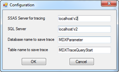
  3. Double-click MDXParameter.exe to start it. You will be prompted to specify the connection details. Note that MDXParameter will automatically create the table schema.

111111_1320_MDXParamete1

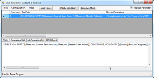
  1. Click OK to launch the main interface and click Start to start the trace.
  2. Go to your SSRS report and run it. Make sure to delete the *rdl.data file in the SSRS project folder to avoid running the report with cached datasets.
  3. Click Stop to stop the trace. You should see the all report MDX queries captured. Select a query to see its statement in the MDX tab. If the query has parameters, MDXParameter will replace them with the actual values (if the Replace Parameter checkbox is selected). This of course is the main reason why you need MDXParameter as it saves you a great deal of time if you want to execute the query with many parameters in SSMS. The tabParametersGrid shows you a grid with the actual parameter values. The Execute MDX button is currently not functioning.

111111_1320_MDXParamete2

MDXParameter supports SSAS 2005, 2008, and R2.

Partition Generator for Multidimensional Cubes

Today happens to be my birthday. To reverse the tradition, how about I give you a gift? If you find yourself spending hours creating partitions in BIDS, you might find the Partition Generator sample (requires registration at the Prologika website) useful. Often, I partition larger cubes by month which may require creating quite a few partitions. Not only is this time-consuming and tedious, but is also error-prone as you can easily get the partition slice query wrong. Written as a C# console application, Partition Generator has the following design goals:

  1. Keep it simple on purpose and due to time constraints. So, no GUI yet and you need to have basic .NET coding skills. You will need Visual Studio 2008 or later with C# to configure it.
  2. Auto-generate a partition definition file in an offline mode without making changes to the server by default. You can use this file to replace the *.partitions file in BIDS so the partitioning scheme can become a part of your project.
  3. Support an online mode where you can deploy the partition changes to the server.

Configuring Partition Generator

Configuring partition generator requires opening the source and making changes to reflect your environment. Specifically, you need to update the following variables:

static string _server = “<your server>”; // SSAS server where the cube is deployed

static string _database = “<database>”; // SSAS datasbase

static string _cube = “<cube>”; // SSAS cube to partition

static string _measureGroup = “<measure group>”; // Measure group to partition

static string _dataSource = “<data source name>”; // The data source name

static DateTime _dateStart = new DateTime(2007, 1, 1); // start date for the period

static DateTime _dateEnd = new DateTime(2020, 12, 31); // end date for the period

// the partition query

static string _query = SELECT * FROM [dbo].[FactInternetSales] WHERE OrderDateKey ;

Note that you need a live cube to connect to which can be partitioned or not partitioned (default partition only). The start date and end date variables specify the start date for the first partition and end date for the last partition respectively. By default, Partition Generator will partition by month but you can overwrite this in code by changing the following line:

_dateStart = _dateStart.AddMonths(1); // assuming parititon by month

Partition Manager creates also start and end partitions for dates outside the date range which could be handy if you forget to add partitions after the end date is passed. Partition Generator sets also the partition slice which is a recommended performance-optimization technique.

Updating the Project

Once you configure Partition Generator, run it with Ctrl+F5. It uses AMO to retrieve the cube metadata and generates a partitions.xmla file in the project bin\debug folder.

  1. Double-click the partitions.xmla to open it in SQL Server Management Studio.
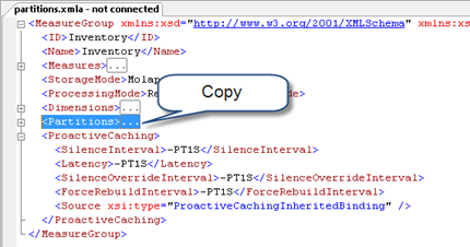
  2. Find and collapse the Partitions XML element. Select the Partitions element and press Ctrl+C to copy its content.

    102411_2129_PartitionGe1


  3. Back up your SSAS project. Open your SSAS project in BIDS. In Solution Explorer, click Show All Files.
  4. Expand the Cubes folder, right-click the <cube name>.partitions file and click View Code to open its source.
  5. Find and select the entire Partitions element for the measure group you want to partition,  and press Ctrl+V to replace the source with new partition schema which you copied in SSMS.
  6. Save the project and close BIDS. That’s because BIDS doesn’t handle well changes made directly to the source files.
  7. Open the SSAS project again in BIDS. Open your cube in the Cube Designer and click the Partitions tab. You should see the new partitions.

Deploying Partitions

By default, Partition Generator doesn’t change the deployed cube. It reads metadata only. However, you can be configured to deploy the partition changes. This could be useful when you want to experiment with different partitioning schemes, such as by month, quarter, year, etc. To configure Partition Manager to deploy the changes:

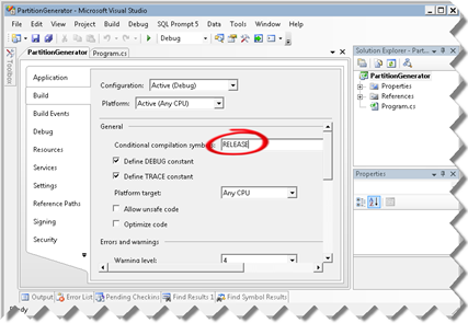
  1. In the PartitionGenerator project, right-click the PartitionGenerator project node in Solution Explorer and click Properties.
  2. In the Project Properties dialog box, select the Build tab and define a RELEASE conditional compilation symbol as follows:

    102411_2129_PartitionGe2

  3. Run Partition Manager to generate both the partitions.xmla file and apply the changes to the SSAS server.

I haven’t tested Partition Manager with BISM Tabular. It should work since Tabular uses the same Partition element in the model (*.bim) file. One more thing – Partition Manager is not supported so please use it at your own risk.

Enjoy!

BISM Tabular Dynamic Data Security Over Bridge Table

About four years ago, in my article Protect UDM with Dimension Data Security, I introduced an approach to secure dimension data in multidimensional cubes by using a factless bridge table. Since then, many BI practitioners have favored this approach because of its simplicity, reusability (transactional reports can join to the security table), and performance. Now that organizational tabular projects support data security, I wanted to try it with BISM Tabular. As it turned out, the factless bridge table approach worked out just fine.

Suppose that you’ve build a tabular project on top of the Adventure Works DW database and the SecurityResellerFilter table is the bridge table that stores the resellers that an employee is authorized to view. As shown in the diagram, SecurityResellerFilter has two relationships SecurityResellerFilter[EmployeeKey] and Employee[EmployeeKey] and SecurityResellerFilter[ResellerKey] and Employee[ResellerKey]. You’d probably want to hide the SecurityResellerFilter table so the end users can’t browse it.

092811_1402_BISMTabular1

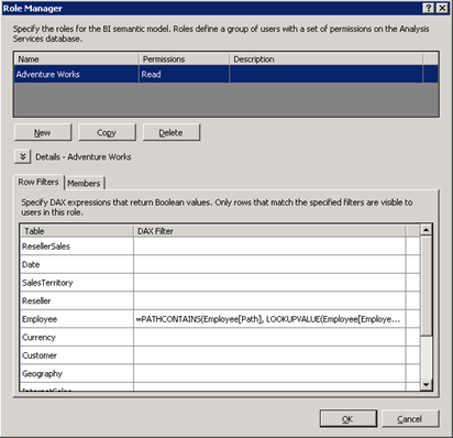
Given this model, implementing a dynamic data security over SecurityResellerFilter requires setting up a new role (click the Roles button in the Analysis Services toolbar) that uses a row filter.

092811_1402_BISMTabular2

A row filter defines a filter expression that evaluates which rows the role is allowed to see. To set up a row filter in the Role Manager, enter a DAX expression next to the table name. The DAX expression must be a Boolean expression that returns TRUE or FALSE. The Adventure Works role uses the following DAX expression for the row filter on the Employee table:

=CONTAINS(RELATEDTABLE(SecurityResellerFilter), SecurityResellerFilter[EmployeeKey], LOOKUPVALUE(Employee[EmployeeKey], Employee[LoginID], USERNAME()))

The LOOKUPVALUE function is used to obtain the employee key associated with employee’s Windows login which we get from the Username function. Because the row filter is set on the Reseller table, for each reseller the CONTAINS function attempts to find a match for the combination of the reseller key and the employee key. Notice the user of the RELATEDTABLE function to pass the current reseller. The net effect is that the CONTAINS function returns TRUE if there is a row in the SecurityResellerFilter table that matches the ResellerKey and EmployeeKey combination.

You can use the Analyze in Excel feature (click the Analyze in Excel button in the Analysis Services toolbar) to test the security changes. To verify that the user has access only to resellers the user is authorized to see, add the ResellerName field from the Reseller table in the Column Labels zone.

092811_1402_BISMTabular3


The report should show on columns only the resellers that are associated with the interactive user in the SecurityResellerFilter table.

Cube vs. VertiPaq Query Performance

This is a big topic and frankly it’s too ambitious on my part to tackle it. Assuming equivalent multidimensional (BISM Multidimensional) and tabular (BISM Tabular) models, I was curious how a multidimensional cube fares against VertiPaq in terms of performance. To be fair to VertiPaq, I decided to use native DAX queries. As you’ve probably heard, BISM Tabular in SQL Denali will include a variant of DAX to query tabular models deployed to SharePoint and SSAS running in VertiPaq mode. Chris Webb has a good writeup about DAX queries here. The DAX EVALUATE construct allows external clients to query tabular models using native DAX syntax instead of MDX. Since BISM Tabular speaks DAX, DAX queries are likely to be more efficient and give you better performance when querying tabular models. At this point, only Crescent generates native DAX queries. The DAX query syntax is:

DEFINE

MEASURE Table1 [measure1] = <DAX_Expression>

MEASURE Table2 [measure2] = <DAX_Expression>

EVALUATE <DAX Table Expression>

ORDER BY

    <DAX_Expression> [ASC | DESC]

    <DAX_Expression> [ASC | DESC]

START AT

    Value_or_Parameter, Value_or_Parameter, …

To have a more sizable dataset, I used the Contoso cube for my tests. I created a BISM Tabular model and imported the Contoso data. Since you probably don’t have Contoso, I provide queries that target the Adventure Works cube. I’ve started with the following unoptimized MDX query which calculates the average sales amount by date across products whose daily sales exceed the daily sales for the same date in the previous month:

WITH


MEMBER [Measures].SlowAvg AS


Avg

(


Filter

(

[Product].[Product].[Product].MEMBERS

,[Measures].[Sales Amount] > ([Measures].[Sales Amount], ParallelPeriod([Date].[Calendar].[Month]))

)

,[Measures].[Sales Amount]

)

SELECT

[Measures].SlowAvg ON 0,

[Date].[Calendar].[Date].Members
ON 1

FROM [Adventure Works];

Then, I optimized the query to take advantage of block computation mode, as follows:

WITH


MEMBER diff as
iif ([Measures].[Sales Amount] > ([Measures].[Sales Amount], ParallelPeriod([Date].[Calendar].[Month])), [Measures].[Sales Amount], null)


MEMBER [Measures].SlowAvg AS


Avg

(

[Product].[Product].[Product].MEMBERS, diff

)

SELECT

[Measures].SlowAvg ON 0,

[Date].[Calendar].[Date].Members
ON 1

FROM [Adventure Works];

Finally, my equivalent DAX query that used to measure performance was:

define measure FactResellerSales[TotalSales] = Sum([SalesAmount])

measure FactResellerSales[TotalSales – LastYear] = [TotalSales](SamePeriodLastYear(DimDate[FullDateAlternateKey]), All(DimDate))

measure FactResellerSales[AverageSales] = AverageX(Filter(Values(DimProduct[ProductKey]), [TotalSales] > [TotalSales – LastYear]), [TotalSales])

evaluate addcolumns(filter(values(DimDate[DateKey]), not isblank([AverageSales])), “AverageSalesAmount”, [AverageSales])

order by [DateKey]

And, the findings from the tests:

1.       MDX query un-optimized (cell calculation model) both on cold cache and executed second time – 33 sec

2.       MDX query optimized (block computation mode) on cold cache – 4.8 sec

3.       MDX query optimized (block computation mode) executed second time – 0.7 sec

4.       DAX query both on cold cache and executed second time – 6.4 sec

Here are some take-home notes:

  1. The fact that VertiPaq is an in-memory database doesn’t mean that it will perform much better than a multidimensional cube. The formula engine of BISM Multdimensional does cache query results in memory. So does the Windows OS. In fact, the more the cube is used, the higher the chances that its data will end up in memory.
  2. VertiPaq might give you good performance without special tuning. All DAX calculations run in a block computation mode.
  3. Optimized MDX queries might outperform VertiPaq especially if results are cached.
  4. DAX queries are never cached which explains why DAX queries perform the same when executed subsequently.

The fact that VertiPaq gives you a head start doesn’t mean that you cannot write inefficient DAX queries. For example, the following DAX measure definition returns the same results but it’s twice as slow.

measure FactResellerSales[AverageSales] = AverageX(Filter(AddColumns(Values(DimProduct[ProductKey]), “x”, [TotalSales]), [x] > [TotalSales – LastYear]), [x])

Again, this is an isolated test case and your mileage might vary greatly depending on queries, data volumes, hardware, etc. But I hope you could use it as a starting point to run your own tests while waiting for a VertiPaq performance guide.

Using the IF Operator in Scope Assignments

UDM scope assignments are incredible useful because they let you write to the cube space, such as to implement custom aggregation, allocations, currency conversion, data calculations, and so on. Unfortunately, scope assignments have limitations. One of them is that more complicated scope expressions result in “an arbitrary shape of the sets is not allowed in the current context” error. Recently, I tried to use a scope assignment to zero out a cube subspace that the end user shouldn’t see and cannot be protected via dimension data security. I tried the following scope assignment (translated to Adventure Works):

Scope (

Employee.Employees.Members – Exists([Employee].[Employees].Members, <another set>, “<Measure Group Name>”),

<another attribute hierarchy>

);

this = null;

End Scope;

This produces the above error caused by employee set expression and as far as I know there is nothing you can do to rewrite the scope expression to avoid the error. In a moment of Eureka, I recall the IF operator and rewrote the scope as:

Scope (

<another attribute hierarchy>

);

IF Intersect([Employee].[
Employees].CurrentMember,

Exists([Employee].[Employees].Members, <another set>, “Measure Group Name”)

).Count = 0 THEN

this = null

END IF

End Scope;

This worked and appears that it performs well. But knowing better about scope assignments I was concerned that there might be hidden performance traps ahead. Jeffrey Wang from the Analysis Services was king enough to provide some input and even write a detailed blog about the performance implications of the IF operator. BTW, you are missing a lot if you are not following Jeffrey’s MDX and DAX blog.

As it turned out, the philosophical answer about the IF performance impact is “it depends”. Let’s say you have another scope assignment X. Instead of calculating X directly, you will be calculating something like IIF(not condition, X, NULL). So we are talking about extra overhead of an IIF function which can deliver good performance if X is in block mode. The bottom line is the server will try to apply block mode logic for IF statements. In my case, the condition would result in cell-by-cell mode but I might still get good performance if the other scope assignment (X) operates in block mode.

Although initially it appeared that there isn’t performance impact in my case, more testing revealed a severe performance hit. The cube had also scope assignments for currency conversion. These assignments interfered with the IF logic and the cube performance took a big hit. Consequently, I had to scratch out this approach.

I hope Jeffrey will write a new blog about what causes the very annoying “an arbitrary shape of the sets is not allowed in the current context” and how to avoid it if possible.