Posts

Divorce Your Methodology

At the Atlanta BI meeting last night, there was a question from the audience about differences between Inmon and Kimball and which methodology should be followed when implementing a data warehouse. I’ll recapture my thoughts and the feedback I shared.

As BI practitioners, most of us use methodologies and it’s easy to fall in love with a specific methodology. But sometimes methodologies conflict each other. So, don’t feel very strongly about methodologies. Instead, study them and try to synthetize their best. The best methodology is the one that delivers a business solution in the most practical and simple way. Back to Inmon vs Kimball, I have deep respect for both of them. They both contributed a lot to data warehousing that forms the backbone of modern BI. Both of these two methodologies aim to consolidate data and promote a single version of the truth. Both of them are “pure” database-focused and vendor-neutral methodologies for designing data structures. But they also differ in significant ways. This table summarizes the high level differences between the two methodologies.

Inmon Kimball
APPROACH Top-down
Data warehouse first, data marts later
Bottom-up
Data marts first, data warehouse later
SCHEMA Normalized (3NF) schema Denormalized (star) schema
HISTORY All history needs to be captured Depends on business requirements
Type 1 vs Type 2 dimensions


So, which one to follow? My answer is that there is a place for both. Consider the following BI architectural view.

012914_0241_DivorceYour1

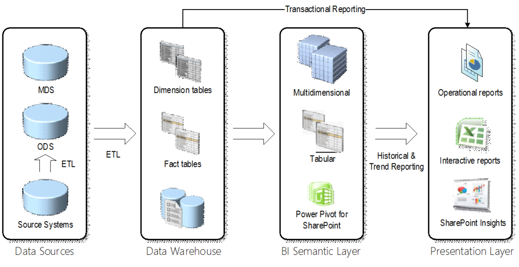
Data comes from veriety of data sources. Some data, such as Products, Customers, Organizations, represents master data that should be ideally maintained in a separate repository, e.g. in Master Data Services. However, most of the source data is not master data and must be staged before it’s imported in the data warehouse. Instead of a transient staging database whose data is truncated with each ETL run, consider an ODS-style staging database that maintains historical changes.

Start_Date End_Date Store Product Deleted_Flag
1/1/2010 5/1/2010 Atlanta Mountain Bike 1
5/2/2010 3/8/2012 Atlanta Mountain Bike 2
3/9/2012 12/31/9999 Norcross Mountain Bike 2

The Start_Date and End_Date columns are used to record the lifespan of each record and create row new versions each time the source row is changed. The example shows three changes that a given product has undergone. This design offers two main benefits:

1.    It maintains a history of all changes that were made to all columns to all tables. Typically, OLTP systems don’t keep track of changes so the staging database can be used to record changes.

2.    It maintains a full backup of the data. If a data warehouse needs to be reloaded, its history can be recreated from the staging database.

This ODS design is effectively your Inmon methodology in practice. For the data warehouse, I’d go with Kimball dimensional modelling. Dimensional modelling is a practical design technique whose goal is to produce a simple schema that is optimized for reporting. As far as data marts, I’m not so excited about moving data in or out of the data warehouse. In most cases, the most practical approach would be to implement a single data warehouse database and extend it as more subject areas come onboard. However, large organizations might benefit from data marts. For example, a large organization might have an enterprise data warehouse but for whatever reasons (usually IT not having enough resources), it might be difficult or not practical to extend it with a new subject areas. Then, this department might spin off its own data mart, such as on a separate database server (even from a different vendor, e.g. DW on Oracle and DM on SQL Server).

Ideally, the data mart should be able to reuse some of conformant dimensions from the data warehouse instead of implementing them anew. In reality, though, the enterprise bus could remain a wishful thinking. Having been left on his own devices, that department would probably need to implement the dimensions from the data they work with. For example, if this is an HR data mart, they would probably source an Organization dimension from PeopleSoft which is where their core data might come from.

With the risk of repeating myself, I want to reemphasize the role of the semantic layer which plays a critical role in every BI architecture. If you are successful implementing an enterprise bus consisting of a data warehouse and data marts (hub and spokes architecture), the semantic layer can provide a unified view the combines these data structures. For more information about the semantic layer benefits, refer to my newsletter “Why Semantic Layer“.

Smart Date Keys Got Smarter

Using “smart” date surrogate integer keys in the format YYYYMMDD is a dimensional modeling best practice and venerable design technique. To make them smarter though, consider using the Date data type which was introduced in SQL Server 2008. The Date data type stores the date without the time component which is exactly what you need anyway. Using the Date data type instead of integers have the following benefits:

  • The Date data type allows you to perform date arithmetic easier as the date semantics is preserved, so you can use date functions, such as YEAR and MONTH when querying the table or partitioning a cube.
  • Self-service BI users can conveniently filter dates on import. For example, PowerPivot enables relative date filtering, such as Last Month, when the user filters a date column.
  • The Date data type has a storage of three bytes as opposed to four bytes for integers.

The only small downside of using the Date data type is that you will end up with funny looking unique names for the Date members in your Date dimension in an SSAS cube. The unique name will include the time portion, such as [Date].[Date].&[2013-07-01T00:00:00]. If you construct date members dynamically, e.g. to default to the current date, you have to append the time portion or use the Format function, such as Format(Now(),”yyyy-MM-ddT00:00:00″).

Optimizing Massive SQL Joins

Scenario: Run ETL to perform a full data warehouse load. One of the steps requires joining four biggish tables in a stating database with 1:M logical relationships. The tables have the following counts:

VOUCHER: 1,802,743

VOUCHER_LINE: 2,183,469

DISTRIB_LINE: 2,658,726

VCHR_ACCTG_LINE: 10,242,414

Observations: On the development server, the SELECT query runs for hours. However, on the UAT server it finished within a few minutes. Both servers have the same data and hardware configuration, running SQL Server 2012 SP1.

Solution: Isolating the issue and coming up with a solution wasn’t easy. Once we ruled out resource bottlenecks (both servers have similar configuration and similar I/O throughput), we took a look at the estimated query plan (we couldn’t compare with the actual execution plan because we couldn’t wait for the query to finish on the slow server).

We’ve notice that the query plans were very different between the two servers. Specifically, the estimated query plan on the fast server included parallelism and hash match join predicates. However, the slow server had merge M:M join predicates. This requires a tempdb work table for inner side rewinds which surely can cause performance degradation.

030313_0112_OptimizingM1

Interestingly, the cardinality of the tables and estimated number of rows didn’t change much between the two plans. Yet, the query optimizer decided to choose very different plans. At this point, we figured that this could be an issue with statistics although both servers were configured to auto update statistics (to auto-update statistics SQL Server requires modifications to at least 20% of the rows in that table). The statistics on the slow server probably just happened to have a sample distribution that led to a particular path through the optimizer that ended up choosing a serial plan instead of a parallel plan. Initially, we tried sp_updatestats but we didn’t get an improvement. Then, we did Update Statistics <table name> With Fullscan on the four tables. This resolved the issue and the query on the slow server executed in par with the query on the fast server.

Note: Updating statistics with full scan is an expensive operation that probably shouldn’t be in your database maintenance plan. Instead, consider:

1. Stick with default sampled statistics

2. Try hints for specific queries that exhibit slow performance, such as OPTION (HASH JOIN, LOOP JOIN) to preclude the expensive merge joins.

Special thanks to fellow SQL Server MVPs, Magi Naumova, Paul White, Hugo Kornelis, and Erland Sommarskog for shedding light in dark places!

Gartner’s 2013 Data Warehouse Magic Quadrant

MVP fellow, Andrew Burst, discusses Gartner’s newly released DW (not BI, mind you) magic quadrant. It looks like Gartner fell in love with Teradata but Microsoft is moving up as well thanks to the advances in its Parallel Data Warehouse (PDW) and in-memory offerings.

1106.gartnerBI2013.png-550x0


Analysis Services Processing and CXPACKET Waits

Performance tuning – my favorite! This blog originated from a quest to reduce the processing time of an SSAS cube which loads some 2.5 billion rows and includes DISCINTCT COUNT measure groups. The initial time to fully process the cube was about 50 minutes on a dedicated DELL PowerEdge R810 server, with 256 GB RAM and two physical processors (32 cores total). Both the SSAS and database servers were underutilizing the CPU resources with SSAS about 60-70 utilizations and the database server about 20-30 CPU utilization. What was the bottleneck?

By using the sys.dm_os_waiting_tasks DMV like the statement below (you can use also the SQL Server Activity Monitor), we saw a high number of CXPACKET wait types.

SELECT
dm_ws.wait_duration_ms,

dm_ws.wait_type,

dm_es.status,

dm_t.TEXT,

dm_qp.query_plan,

dm_ws.session_ID,

dm_es.cpu_time,

dm_es.memory_usage,

dm_es.logical_reads,

dm_es.total_elapsed_time,

dm_es.program_name,

DB_NAME(dm_r.database_id) DatabaseName,

— Optional columns

dm_ws.blocking_session_id,

dm_r.wait_resource,

dm_es.login_name,

dm_r.command,

dm_r.last_wait_type

FROM
sys.dm_os_waiting_tasks
dm_ws

INNER
JOIN
sys.dm_exec_requests
dm_r
ON
dm_ws.session_id = dm_r.session_id

INNER
JOIN
sys.dm_exec_sessions
dm_es
ON
dm_es.session_id = dm_r.session_id

CROSS
APPLY
sys.dm_exec_sql_text
(dm_r.sql_handle)
dm_t

CROSS
APPLY
sys.dm_exec_query_plan
(dm_r.plan_handle) dm_qp

WHERE
dm_es.is_user_process = 1

The typical advice given to address CXPACKET waits is to decrease the SQL parallelism by using the MAXDOP setting. This might help in some isolated scenarios, such as UPDATE or DELETE queries. However, the SQL Sentry Plan Explorer showed that each processing query is highly parallelized to utilize all cores. Notice in the screenshot below, that thread 16 fetches only 14,803 rows.

051512_0211_AnalysisSer1

Therefore, the CXPACKET waits were simply caused by faster threads waiting for other threads to finish. In other words, CXPACKET wait is just a coordination mechanism between the threads being parallelized. To confirm this, we set the SQL Server MAXDOP setting to 1. Surely, the CXPACKET waits disappeared but the overall cube processing time went up as well. In our case, the biggest benefit was realized not by decreasing the SQL Server parallelism but by increasing it, by increasing the maximum number of database connections. This resulted in decreasing the overall processing time some 20%.

051512_0211_AnalysisSer2

You need to be careful here though. While increasing the connections to max out the CPU on the SSAS server will yield the biggest gain, it might also slow down other processing, such as reports that query the cube while the database is being processed. So, as a rule of thumb, target no more than 80% CPU utilization to leave room for other tasks.

Columnstore Indexes To Speed ETL

SQL Server 2012 introduces columnstore indexes. Using the same in-memory VertiPaq engine that powers PowerPivot and Analysis Services Tabular, columnstore indexes can speed up dramatically SQL queries that aggregate large datasets. For a great introduction to columnstore indexes, see the video presentation, “Columnstore Indexes Unveiled” by Eric Hanson. I personally don’t see columnstore indexes as a replacement of Analysis Services because an analytical layer has much more to offer than just better performance. However, in a recent project we’ve found a great use of columnstore indexes to speed up ETL processes.

Issue: Perform an initial load of a snapshot fact table for inventory analysis from another fact table with one billion rows. For each day, extract some 200 million rows from the source fact table and group these rows into a resulting set of about 300,000 rows to load the snapshot fact table for that day. The initial estimates indicated that that the extraction query alone takes about 15 minutes when using a clustered index. And, that’s just for one day. Given this speed, we estimated the initial load could take weeks.

Solution: We upgraded to SQL Server 2012 and created a columnstore index on selected columns from the source fact table. We excluded high-cardinality columns that were not used by the extraction query to reduce the size of the index. Creating the index on the source table (1 billion rows) took about 10 minutes and this is very impressive. The disk footprint of the index was about 4GB. We ran the same extraction query and saw a five-fold performance improvement. This query, which would previously run for 15 minutes with a B-tree clustered index, would now finish in 3 minutes with a columnstore index.

When testing your queries with columnstore indexes, it is important to make sure that the query executes in Batch mode. As you can see in the screenshot below, the query uses the columnstore index and the execution mode is Batch. If it says Row, the query performance degrades significantly. Watch Eric Hanson’s presentation to understand why this happens and possible workarounds.

120811_0048_Columnstore1

When I did initial tests to test the columnstore index, I ran into a gotcha. I tested a simple “SELECT SUM(X) FROM TABLE” query to find that it executes in a Row mode and the query took about 2 minutes to finish. As usual, the first thing I try doesn’t work. As it turned out, currently a columnstore index doesn’t support batch mode with scalar aggregates. You need to rewrite the query with a GROUP BY as Eric Hanson explains this in more details in his blog, “Perform Scalar Aggregates and Still get the Benefit of Batch Processing”. This is rather unfortunate because every ad-hoc report starts with the end user dropping a measure and the report tool generating such queries.

When testing the performance gain, it’s useful to compare how the same query would perform without a columnstore index. Instead of having two tables or dropping the index, you could simply tell SQL Server to ignore the columnstore index, such as:

SELECT … FROM…WHERE…GROUP BY…

OPTION (IGNORE_NONCLUSTERED_COLUMNSTORE_INDEX)


To sum up, when you are pushing the envelope of traditional B-tree indexes and queries aggregate data, consider SQL Server 2012 columnstore indexes. The query optimizer would automatically favor a columnstore index when it makes sense to use it. Columnstore indexes require a read-only table but the cost of dropping and recreating them is not that high. Or, you could add them to speed up the initial DW load and drop them once the load completes.


Disabling Foreign Key Constraints

Disabling check constraints, such as foreign key constraints, is often required when populating a data warehouse. For example, you might want to disable a check constraint to speed up loading of a fact table.

  1. How do we disable check constraints in SQL Server?
    You can script each check constraint or you can use the undocumented sp_MSforeachtable function.

    ALTER
    TABLE [dbo].[FACT_ITEM_INVENTORY] NOCHECK
    CONSTRAINT [FK_DIM_DATE_FACT_ITEM_INVENTORY_Date_Id] — disables a specific contraint

    sp_MSforeachtable
    ‘ALTER TABLE ? NOCHECK CONSTRAINT ALL’ — disables all contraints in the database

    Once the foreign keys are disabled, you can run the ETL job or delete records from the referenced table without referential integrity checks. Note that you cannot truncate a table even if you have disabled the constraints due to the different way SQL Server logs the truncate operation. You must drop the constraints if you want to truncate a table. You can use sp_MSforeachtable to drop constraints as well although I personally prefer to disable them for a reason that will become obvious in a moment.

  2. How do we enable check constraints?

The same way you disabled them but this time you use the CHECK predicate:

ALTER
TABLE [dbo].[FACT_ITEM_INVENTORY] CHECK
CONSTRAINT [FK_DIM_DATE_FACT_ITEM_INVENTORY_Date_Id] — enables a specific constraint

sp_MSforeachtable
‘ALTER TABLE ? CHECK CONSTRAINT ALL’ — enables all contraints in the database

  1. Does SQL Server verify referential integrity for existing data when you re-enable check constraints?

    This is where the behavior differs between recreating and enabling constraints. If you drop and create the constraints, the server will check the data unless WITH NOCHECK is used.

    ALTER
    TABLE [dbo].[FACT_ITEM_INVENTORY] WITH
    NOCHECK

    ADD
    CONSTRAINT [FK_DIM_DATE_FACT_ITEM_INVENTORY_Date_Id] FOREIGN
    KEY([Date_Id]) REFERENCES [dbo].[DIM_DATE] ([Date_Id])

    The server doesn’t check existing data if you enable a previously disabled constraint. You can manually check foreign key violations by using this command:

    dbcc
    checkconstraints(FACT_ITEM_INVENTORY) –- checks a specific table

    dbcc
    checkconstraints — checks the entire database

The checkconstraints command will output all rows that violate constraints.

UPDATE 10/31/2011

Reader Ian pointed out that re-enabling foreign key constraints without checking data marks them as non-trusted. Consequently, the SQL Server optimizer may choose different execution plans for a certain range of queries. Tibor Karaszi explains this in more details in his blog Non-trusted constraints and performance. Paul White also mentions about a bug in this area. This makes me believe that enabling check constraints without checking data should be avoided. Therefore, to speed up fact table imports for large dataset consider:

  1. Disable foreign key constraints
  2. Drop indexes on fact tables
  3. Import data
  4. Recreate indexes on fact tables
  5. Re-enable constraints with the WITH CHECK option


sp_MSforeachtable

‘ALTER TABLE ? WITH CHECK CHECK CONSTRAINT ALL’ — enables all constraints in the database