How to Test SSRS Data Alerts without Corporate Mail Server

Reporting Services data alerts were introduced in SQL Server 2012 to allow business users to receive e-mail notifications based on rules they specify. Data alerts require SSRS to be configured in SharePoint integration mode. However, you’d probably run SharePoint on a VM for development and demo purposes and you might not have access to a functional mail server. The following steps allow you to configure your VM to test data alerts with a local SMTP server:

  1. Assuming your SharePoint VM is running Windows Server 2012, open Turn Windows Features On and Off and add the SMTP Server feature. This will install a local SMTP server.
  2. Open IIS Manager 6.0 and start the SMTP Virtual Server. Configure the SMTP server to allow relay.
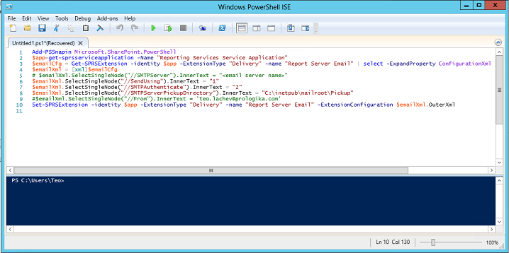
  3. Because SSRS 2012 integrates natively with SharePoint, you can’t use the report server configuration files to directly change the SSRS settings. Instead, you must use PowerShell as I explained here. Open Windows PowerShell ISE and execute the following script to configure the SSRS e-mail settings. Replace <your SSRS application name> with the name of your SSRS application which you can obtain from the SharePoint Central Administration ð Manage Service Applications. Execute the script.

    051014_2250_HowtoTestSS1

    Add-PSSnapin Microsoft.SharePoint.PowerShell

    $app=get-sprsserviceapplication -Name “<your SSRS application name>”

    $emailCfg = Get-SPRSExtension -identity $app -ExtensionType “Delivery” -name “Report Server Email” | select -ExpandProperty ConfigurationXml

    $emailXml = [xml]$emailCfg

    # $emailXml.SelectSingleNode(“//SMTPServer”).InnerText = “<email server name>”

    $emailXml.SelectSingleNode(“//SendUsing”).InnerText = “1”

    $emailXml.SelectSingleNode(“//SMTPAuthenticate”).InnerText = “2”

    $emailXml.SelectSingleNode(“//SMTPServerPickupDirectory”).InnerText = “C:\inetpub\mailroot\Pickup” # You probably don’t need this; I was experimenting with dropping the messages to a pickup folder

    $emailXml.SelectSingleNode(“//From”).InnerText = ‘teo.lachev@prologika.com’

    Set-SPRSExtension -identity $app -ExtensionType “Delivery” -name “Report Server Email” -ExtensionConfiguration $emailXml.OuterXml

  4. If you haven’t configured the data alerts before, go to SharePoint Central Administration ð Manage Service Applications ð <Your SSRS Application>, and then click Provision Subscriptions and Alerts. If you have admin permissions to the SQL Server that hosts the SharePoint databases, enter your credentials and click OK to grant the SSRS service account access to the SQL Server Agent (the SQL Server Agent Service must be running for the data alerts to work). If you don’t, then click the Download SQL Script link and give the script to the DBA to execute the script in order to grant the SSRS service account these permissions.
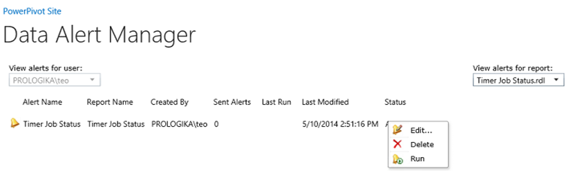
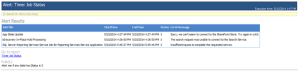
  5. Now, create a data alert as usual and run it from the Manage Data Alerts page. After you manually run the alert, you shouldn’t see an error in the Status column.051014_2250_HowtoTestSS2
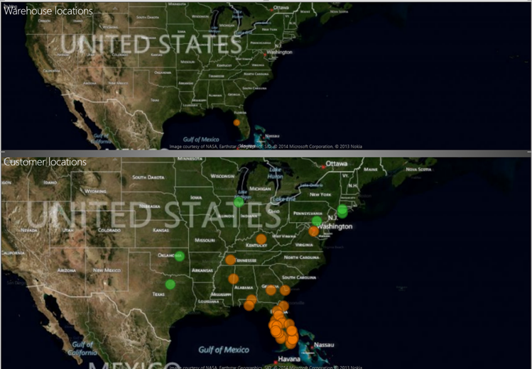
  6. Go to the SMTP service queue folder, the default one is C:\inetpub\mailroot\Queue. You should see files with extension *.EML. You can open these files with Microsoft Outlook to see the details of the e-mail notification that SSRS sends to the recipient. It should look like the one below. In this case, I’ve create a report that shows the status of the SharePoint timer jobs and I wanted to be notified every time the Status=3.

051014_2250_HowtoTestSS3

Point-to-point Geo Adventures

Scenario: You need to visualize point-to-point geospatial data, such as routes from an origin location to destinations. The map region in Reporting Services (Report Designer or Report Builder) supports point-to-point mapping but more than likely your users would prefer an interactive report. As they stand, neither Power View nor Power Map support point-to-point mapping. Further down on the limitation list, Power View doesn’t support layers while Power Map does support layers but doesn’t support filtering, e.g. to allow the end user to select a specific origin. Point-to-point mapping is a frequently requested feature which I hope Microsoft will implement in a not so distant future. Meanwhile, you need to resort to workarounds.

Workaround 1: If all the user wants to see is how far the destinations are located relative to a specific origin, consider creating a Power View report with two maps. The first map would allow the user to filter the origin and second map would plot the associated destinations. In the report below, the user has filtered a specific warehouse which is plotted on the first map. The second map shows the locations of the customers who receive shipments from that warehouse.

050514_0022_Pointtopoin1

The following screenshot show you how the first and second maps are configured:

050514_0022_Pointtopoin2

Workaround 2: If you prefer plotting both the origin and destinations on a single map, consider modifying your input dataset (Power Query can help automating this so you don’t have to do it manually) to append the distinct set of origins so you end up with both origins and destinations sharing the same latitude and longitude columns. In other words, you’ll append the origin set consisting of a distinct set of origins one more time to the original dataset. Then, you might want to introduce a Type column, e.g. with values Warehouse and Customer, to denote the type of each row. So that the origin stands out on the map, consider adding a DAX calculated column that does a distinct count over the destinations associated with that origin and use this column for the bubble size. Assuming a single dataset, this calculated column might use the following expression:

Customer Count:=IF([Type]=”Warehouse”, CALCULATE(DISTINCTCOUNT([Customer ID]), ALLEXCEPT(Table1, Table1[Warehouse ID])),BLANK())

Then, the map report can plot both origin and destinations.

050514_0022_Pointtopoin3

The following screenshot shows how the map is configured.

050514_0022_Pointtopoin4

SQL Server Events in Atlanta

Next week will be SQL Server-intensive and your humble correspondent will be heavily involved:

  • Monday, April 28th: Power BI presentation by Brian Jackson, Microsoft for Atlanta MS BI Group with Pyramic Analytics sponsoring the event. This presentation will cover new and compelling Power BI features including: the data manipulation of Power Query, Power BI Sites, the Data Steward Experience, natural language BI using Power Q&A, and mobile BI functionality. There will also be a technical discussion of the Power BI architecture as it relates to authentication, storage, data refresh and the concept of self-service information management.
  • Friday, May 2nd: Three SQL Saturday precon sessions (Deep Dive into the Microsoft BI Semantic Model by Teo Lachev, SQL Performance Tuning & Optimization by Denny Cherry, and What the Hekaton!? A Whole New Way to Think About Data Mgmt by Kalen Delaney). Ping Stuart Ainsworth on Twitter at @codegumbo for $20 discount!
  • Saturday, May 3rd: SQL Saturday – a full day event of top-notch SQL Server sessions. Last year we had a worldwide record attendance with some 570 people attending the event. Help us to top it off this year!

Besides the BISM precon, I’ll do a session a SQL Saturday “Predictive Analytics for the Data Scientist and BI Pro” on May 3rd at 8:15.

“The time for predictive analytics to go mainstream has finally come! Business users and BI Pros can use the Microsoft SQL Server and Microsoft Office to unleash predictive analytics and unlock hidden patterns. Join this session to learn how a data scientist can use the Excel Data Mining add-ins to perform predictive analytics with Excel data. I’ll provide also the necessary fundamentals for understanding and implementing organizational predictive models with Analysis Services.”

042214_1235_SQLServerEv2

Starting SSIS 2012 Job Remotely

Scenario: Inspired by the new SSIS 2012 capabilities, you’ve managed to convince management to install SSIS 2012 on a new server for new ETL development. But your existing ETL is still on SQL Server 2008 (or R2) and there is no budget for migration and retesting. You want to start SSIS 2012 jobs from the 2008 server, e.g. in SQL Server Agent on completion of a certain SSIS 2008 job.

Solution: Courtesy to Greg Galloway for clueing me on this, thanks to its CLR integration, SSIS 2012 supports initiating jobs via stored procedure in the SSIS catalog. Although the process could benefit from simplification, it’s easy to automate it, such as (you guessed it) with an SSIS 2008 calling package. It goes like this:

  1. Call catalog.create_execution in the SSISDB database to create an execution for the SSIS job. At this point, the job is not started. It’s simply registered with the SSIS 2012 framework. Notice that you want to get back the execution id because you will need it for the next calls.

EXEC catalog.create_execution

@folder_name=N'<SSIS Catalog Folder>’,

@project_name=N'<project name>’,

@package_name=N’package name’,

@reference_id=NULL,

@execution_id=? OUTPUT

Note: If you use SSIS 2008 and you declare the variable that stores execution_id (which is a big integer) to be Int64, SSIS 2008 would probably choke due to a known issue with big integers. As a workaround, change the SSIS variable type to Int32.

  1. So that the SSIS 2008 job waits for the SSIS 2012 job to complete, set the Synchronous parameter.
    EXEC catalog.set_execution_parameter_value @execution_id = ?

    ,@object_type=50 ,@parameter_name=’SYNCHRONIZED’

    ,@parameter_value=1

  2. Now you are ready to start the job by calling catalog.start_execution and wait for it to finish.
    EXEC catalog.start_execution @execution_id = ?

  • To get the back the job status, query the status field from the [catalog].[executions] view. A status of 4 means that the job has failed.
    SELECT [status] FROM [SSISDB].[catalog].[executions] WHERE execution_id = ?


  • To get the actual error, query the [catalog].[event_messages] view, e.g.:
    SELECT TOP 1 cast([message] as nvarchar(500)) as message, cast ([execution_path] as nvarchar(500)) as execution_path

    FROM [catalog].[event_messages]

    WHERE operation_id = ? AND event_name = ‘OnError’

    ORDER BY message_time DESC

Tip: If you use SQL Server Agent to start the SSIS 2008 job, use a proxy account to execute the job under a Windows service account that has the required permissions to the SSISDB catalog to start SSIS 2012 jobs.

How to Cluster Analysis Services

Some scenarios require a fault-tolerant SSAS installation. In a real-life project, an active-active cluster met this requirement. Instead of installing an active-passive cluster where one node just plays a sitting duck waiting for the active node to fail, with the active-active cluster we had two active nodes to distribute processing and achieve high availability. The first node had the SQL Server database engine hosting the data warehouse database while the second had SSAS. If one of the nodes would fail, its services will fail over to the other.

Configuring a failover cluster requires many steps. Luckily, Microsoft just published a whitepaper “How to Cluster SQL Server Analysis Services” by Allan Hirt (SQL Server MVP) that includes step-by-step instructions of how to configure SSAS (Multidimensional or Tabular) on a Windows Server failover cluster (WSFC). Although not discussed, instead of WSFC, yet another way to achieve high tolerance that gains popularity is to use VM failover capabilities.

BISM Drillthrough Capabilities

All the three BISM flavors (Multidimensional, Tabular, and Power Pivot) supports default drillthrough to allow the end user to see the level of details behind an aggregated measure by just double-clicking the cell. However, the implementation details differ. Multidimensional supports default drillthrough on regular measures only, that is, measures that bind to columns in fact tables. Multidimensional doesn’t support drillthrough on calculated measures, even if these measures are simple tuples, such as ([Measures].[Sales Amount], [Product].[Product Category].[Some Category]).

On the other hand, Power Pivot and Tabular don’t have the concept of regular measures and they support only calculated measures. Even if the user drags a column to the Values zone on a pivot or Power View report, the tool creates an implicit measure with a DAX formula behind the scenes, such as =SUM(ResellerSales[Sales Amount]). Because of this, Power Pivot and Tabular appears to allow drillthrough on any measure. However, the drillthough action only picks the filter context. It does not parse the calculated measure. So, if you have an explicit measure with a DAX formula that filters the results, such as =CALCULATE( SUM( ResellerSales[Sales Amount] , FILTER(SalesTerritory, SalesTerritory[Country] = “USA” ) ), the drillthrough action won’t return the rows where country=’USA’. Instead, it will return the rows from the ‘home’ table within the default context inferred by rows, columns, and filters on the report.

While we are on the subject of drillthrough, Multidimensional allows the modeler to specify custom actions, such as an action that runs an SSRS report or opens a web page. As it stands, Power Pivot and Tabular don’t provide UI for custom actions although the drillthrough functionality is there. As a workaround, you can use the BIDS Helper Tabular Actions Editor feature to implement custom drillthrough actions.

The Power Pivot Update Story

The Power Pivot update story is somewhat convoluted. Excel 2013 integrates Power Pivot natively and the only way to get it updated (assuming the traditional MSI installation option) is through Office updates because the Office team now owns its distribution. Alternatively, if you have an Office 365 subscription, and have installed Office 2013 via the click-to-run option, then the Office and Power Pivot updates will be pushed to you automatically.

With Excel 2010, Power Pivot is an external add-in that can be updated from the Microsoft download center. While the Excel 2013 Power Pivot bits are installed in the %Program Files%\Microsoft Office\Office15\ADDINS\PowerPivot Excel Add-in, the Excel 2010 Power Pivot add-in is installed in a different location: %Program Files%\Microsoft Analysis Services\AS Excel Client\110.

The interesting side effect is that the Excel 2010 Power Pivot can be updated more frequently (for example, every time there is a SQL Server 2012 service pack or cumulative update), while Excel 2013 MSI users must wait for an office update (distributed via Windows Update for MSI installer) or via O365 updates.

To make the whole story short:

  1. If you have Excel 2010, use the latest Power Pivot bits available on the Microsoft Download Center.
  2. If you have both Excel 2010 and 2013, use the Microsoft Download center to get Excel 2010 updated. Excel 2013 won’t.
  3. If you have Excel 2013 only, wait for Office updates.

5 Tools for Understanding BISM Storage

Recall that the Microsoft BI Semantic Model consists of three flavors: Multidimensional, Tabular, and Power Pivot. The default storage mode of Tabular and Power Pivot is the xVelocity in-memory engine. The default Multidimensional storage is MOLAP. You might want to analyze which objects consume the most storage space. This especially important for Tabular since computer memory is still a scarce resource.

Windows Explorer

The easiest way to get the storage breakdown for Multidimensional and Tabular is to use Windows Explorer and examine the size of the corresponding data folder under the SSAS Data folder, e.g. C:\Program Files\Microsoft SQL Server\MSAS11.TABULAR\OLAP\Data\AdventureWorks Tabular Model SQL 2012.0.db. Unfortunately, Windows Explorer in Windows 7 and 8 doesn’t show the folder size requiring you either to hover on the folder to see its size or to go the folder properties. As a workaround, consider utilities such as HDGraph or Folder Size. Folder Size, for example, pops up a window in Windows Explorer on the side of each folder that has subfolders to show you the folder size. In the case of the AdventureWorks Tabular Model SQL 2012 Tabular database, we can see that Product Inventory table consumes the most space.

041414_0113_5ToolsforUn1

If you drill down the Product Inventory folder and sort by size, you can see the storage breakdown by column.

BISM Server Memory Report

Another way to analyze Tabular and Multidimensional storage in an user-friendly way is to use the BISM Server Memory Report developed by Kasper de Junge (Senior Program Manager at Microsoft).

DMV Views

Behind the scenes, the BISM Server Memory Report uses SSAS DMV Views which expose expose information about local server operations and server health. Specifically, it uses the Discover_object_memory_usage DMV which you can query directly to obtain the same information.

041414_0113_5ToolsforUn2

Power Pivot Macro

If you use Power Pivot, the easiest way to analyze Power Pivot storage in Excel 2013 is to use the Power Pivot macro made available by Kasper de Junge. When you run the macro, it generates Excel pivot report which you can sort by the object memory size. For example, the report below allows us to see the most memory is consumed by CalculatedColumn1 (although xVelocity calculated columns are stored to disk like regular columns, calculated columns are not compressed).

041414_0113_5ToolsforUn3

Power Pivot PowerShell Script

While the above macro relies on Excel 2013 native integration with Power Pivot and only works with Excel 2013, the methodology and PowerShell script developed by Vidas Matelis (SQL Server MVP) works with both Excel 2010 and 2013.

Where is Your Focus?

With all the tremendous interest around BI, new vendors and tools are emerging almost every day. In general, you can approach your BI needs in two ways.

  1. You can try a top-down approach starting with the presentation layer, hoping that a cool data visualization tool and self-service BI will somehow solve your challenges. Lots of vendors out there would love to take you on that path.
  2. You can follow a bottom-up approach that starts with a solid data foundation and semantic layer that enables a single version of the truth and it is supported by most popular visualization tools.

I had the pleasure to teach a class this week for the HR department of one of the largest and most successful companies. They have an ambitious goal to establish a modern data analytics platform in order to gain insights into all aspects of their workforce. Their manager told that they have tried unsuccessfully the top-down approach and multiple vendor tools until they realized that the focus should be on the data first. And, I agree completely. There are no shortcuts.

On this note, join me for a full-day precon session “Deep Dive into the Microsoft BI Semantic Model (BISM)” at SQL Saturday Atlanta on May 2st to find out how the Microsoft BI helps you deliver a modern BI platform, as well as discussing the toolset strengths and challenges.

Data Models for Self-Service BI

The self-service BI journey starts with the business user importing data. With Microsoft Power Pivot, we encourage the user to import tables and create relationships among these tables, similar to what they would do with Microsoft Access. This brings tremendous flexibility because it allows the user to incrementally add new datasets and implement sophisticated models for consolidated reporting, such as for analyzing reseller and internet sales side by side. True, Power Pivot relationships have limitations, including:

  • The lookup table must have a primary key and the relationship must be established using this key. As it stands, Power Pivot doesn’t support multi-grain relationship where the fact table joins the lookup table at a higher grain than the primary key.
  • Many-to-many relationships (such as a joint bank account) are not natively supported and currently require simple DAX formulas to resolve the relationship, such as CALCULATE ( SUM ( Table[Column] ), BridgeTable)
  • Closed loop relationships (Customer->Sales->Orders->Customer) are not allowed, etc.

The chances that these constraints will be relaxed in time as Power Pivot and Tabular evolve to allow you to meet even more involved requirements on a par with organizational BI models.

033014_1952_DataModelsf1

With the recent popularity of other tools for self-service BI tools, I took a closer look at their data features. Tableau, for example, encourages users to work with a single dataset. If the user wants to import data from multiple tables, the user must create table joins to relate the tables before data is imported in order to create a dataset that has all the required data. This probably meets 80% of self-service BI requirements out there although it might preclude consolidated analysis. Suppose you want to analyze reseller sales by customer. With Tableau, you need to join the Customer and ResellerSales tables in order to prepare the dataset and that’s probably OK to meet this requirement. At some point, however, suppose you need to bring also Internet sales which are stored in a separate table. Now you have an issue. If you opt to change the dataset and join the Customer, ResellerSales, and InternetSales, you’ll end up with duplicated data because you can’t join ResellerSales to InternetSales (they don’t have a common field). In Power Pivot, you could simply address this by importing Customers, ResellerSales, and InternetSales as separate tables and creating two relationships Customer->ResellerSales and Customer->InternetSales. Notice that a Power Pivot relationship happens after the tables are imported although it’s possible of course to establish a data source join during the data import. A Tableau workaround for the above scenario would be to go for “data blending”. Speaking of which…

It’s also interesting how Tableau addresses combining data from separate data sources. Referred to as “data blending”, this scenario requires the user to designate one of the data sources as primary and specifying matching fields from the two data sources to perform the join. Behind the scenes, Tableau executes a post-aggregate join that aggregates data at the required grain. Let’s say, you import the Customer table from Data Source A and InternetSales table from Data Source B. Suppose that both the Customer and InternetSales datasets have a State field which you want to use for the join. With data blending, Tableau will first aggregate the InternetSales dataset at the State level (think of SUM(SALES) FROM … GROUP by STATE) and then join this dataset to the Customer dataset on the State field. The advantage of this approach is that you can join any two datasets as long as they have a common field (there is no need for a primary key in the Customer table). The disadvantage is that the secondary data source can’t be joined to another (third) data source. Further, this approach precludes more complicated data entity relationships, such as many-to-many.

When choosing a self-service BI tool, you need to carefully evaluate features and one of the most important criteria is the tool data capabilities. Some tools are designed for one-off analysis on top of a single dataset and might require importing the same data to meet different reporting requirements. Power Pivot gives you more flexibility but requires end users to know more about data modeling, tables and relationships.