Archive for month: August, 2018

A Power BI training or assessment won’t be complete unless I get hammered on the Power BI sharing limitations. So far, I could only mumble something to the extent of “I agree that Power BI sharing sucks big time”, look for the exit and suggest an unplanned break. Fortunately, it looks like quantitative accumulations from unhappy corporate customers have resulted in qualitative changes as Microsoft is getting serious about addressing these limitations. To me, as it stands today, the Power BI sharing is a classic example of overengineering. Something that could have been easily solved with the conventional and simple folders a la SSRS, morphed into some farfetched “cool” vision of workspaces and apps without much practical value. Let’s revisit the current Power BI sharing limitations to understand why change was due:

• Workspace dependency on Office 365 groups – This results in explosion of workspaces as Power BI is not the only app that creates groups.
  
• Any Power BI Pro user can create a workspace – IT can’t put boundaries. I know of an organization that resorted to an automated script that nukes workspaces which aren’t on the approved list.
  
• You can’t add security groups as members – As I discussed in my blog “Power BI Group Security“, different Power BI features have a different degree of support for groups. For example, workspaces didn’t support AD security groups.
  
• Coarse content access level – A workspace could be configured for “edit” or “view only” at the workspace level only. Consequently, it wasn’t possible to grant some members view access while others edit permissions.
  
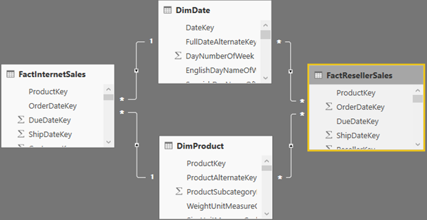
• (UPDATE 6/9/2019: A dataset can now be shared across workspaces) Content sharing limitations – Content can’t be copied from one workspace to another. Worse yet, content can’t be reused among workspaces. For example, if Teo deploys a self-service semantic model to the Sales workspace, reports must be saved in the same workspace. 
• No nesting support – Workspace can’t be nested, such as to have a global Sales workspace that breaks down in to Sales North America, Sales Europe, etc. Again, this is a fundamental requirement that any server-side reporting tool supports but not Power BI. You can’t organize content hierarchically and there is no security inheritance. Consequently, you must resort to a flattened list of workspaces.
• (UPDATE 6/9/2019: A dataset can now be promoted and certified). No IT oversight – There is no mechanism for IT to certify workspace content, such as a dataset. There is no mechanism for users to discover workspace content.
• UPDATE 6/27: The new Viewer role supports sharing with viewers. Sharing with “viewers” – You can’t just add Power BI Free users to share content in a premium workspace. This would have been too simple. Instead, you must share content out either using individual report/dashboard sharing or apps.
• One-to-one relationship with apps – Since broader sharing requires apps (why?), an app needs to be created (yet another sharing layer) to share out workspace content. But you can’t publish multiple apps from a workspace, such as to share some reports with one group of users and another set with a different group.

Enough limitations? Fortunately, the new workspace experience immediately solves the first four (highlighted) issues!

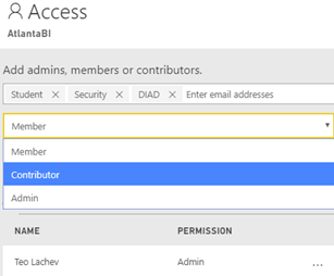
For example, the screenshot below shows how I can add all the O365 group types as members of a workspace (Student is individual member, Security is a security group, and DIAD is a O365 group). Moreover, two new roles, Contributor and Viewer (the Viewer role is not yet available), would further limit the member permissions. So, we finally have member-level security instead of workspace-level security.

What about the other limitations? Microsoft promises to fix them all, but it will take a few more months. Meanwhile, watch the “Distribute insights across the organization with Microsoft Power BI” presentation. So, hopefully by the end of the year I’ll have a much better sharing story to tell after all.

During the “Building a data model to support 1 trillion rows of data and more with Microsoft Power BI Premium” presentation at the Business Applications Summit, Microsoft discussed the technical details of how the forthcoming “Aggregations” feature can help you implement fast summarized queries on top of huge datasets. Following incremental refresh and composite models, aggregations are the next “pro” feature that debuts in Power BI and it aims to make it a more attractive option for deploying organizational semantic models. In this blog, I summarize my initial observations of this feature which should be available for preview in the September release of Power BI.

Aggregations are not a new concept to BI practitioners tackling large datasets. Ask a DBA what’s the next course of action after all tricks are exhausted to speed up massive queries and his answer would be summarized tables. That’s what aggregations are: predefined summaries of data, aimed to speed queries at the expense of more storage. BI pros would recall that Analysis Services Multidimensional (MD) has supported aggregations for a long time. Once you define an aggregation, MD maintains it automatically. When you process the partition, MD rebuilds the partition aggregations. An MD aggregation is tied to the source partition and it summarizes all measures in the partition. You might also recall that designing proper aggregations in MD isn’t easy and that the MD intra-dependencies could cause some grief, such as processing a dimension could invalidate the aggregations in the related partitions, requiring you to reprocess their indexes to restore aggregations. On the other hand, as it stands today, Analysis Services Tabular (Azure AS and SSAS Tabular) doesn’t support aggregations. Power BI takes the middle road. Like MD, Power BI would search for suitable aggregations to answer summarized queries, but it requires more work on your part to set them up.

Consider the following model which has a FactInternetSales fact table and three dimensions: DimCustomer, DimProduct, and DimDate. Suppose that most queries would request data at the Product and Date levels (not Customer) but such queries don’t give you the desired performance. This could be perhaps because FactinternetSales is imported (cached) but it’s huge. Or, FactInternetSales could be configured for DirectQuery but the underlying data source is not efficient for massive queries. This is where aggregations might help (contrary reasons for using aggregations is to compensate for bad design or inefficient DAX).

As a first step for setting up aggregations, you need to add a summarized table. Unlike MD, you are responsible for designing, populating and maintaining this table. Why not the MD way? The short answer is flexibility. It’s up to you how you want to design and populate the summarized table: ETL or DAX. It’s also up to you which measures you want to aggregate. And, the summarized table doesn’t have to be imported (it could be left in DirectQuery). You can also have multiple aggregations tables (more on this in a moment). In my case, I’ve decided to base the FactInternetSalesSummary table on a SQL view that aggregates the FactInternetSales data, but I could have chosen to use a DAX calculated table or load it during ETL. In my case, FactInternetSalesSummary aggregates sales at the Product and Date level, assuming I want to speed up queries at that grain. In real life, FactInternetSalesSummary would be hidden to end users so they are not confused which table to use.

Note that a composite model has specific requirements for configuring dimension tables, which I discussed in my blog “Understanding Power BI Dual Storage“. For example, if FactInternetSalesSummary is imported but FactInternetSales is DirectQuery, DimProduct and DimDate must be configured in Dual storage mode. Once the aggregation table is defined, the next step is to define the actual aggregations. Note that this must be done for the aggregation table (not the detail table) so in my case this would be FactInternetSalesSummary. Configuring aggregations involves specifying the following configuration details in the “Manage aggregations” window:

• Aggregation table – the aggregation table that you want to use for the aggregation design.
• Precedence – in the case of multiple aggregation tables, you can define which aggregation table will take precedence (the server will probe the aggregation table that has a highest level first). Another feature that opens interesting scenarios.
• Summarization function – Supported are Count, GroupBy, Max, Min, Sum, Count. If the aggregation table has relationships to dimension tables, there is no need to specify GroupBy. However, if the aggregation table can’t be joined to the dimension tables in a Many:1 relationship, GroupBy is required. For example, you might have a huge DirectQuery table where all dimension attributes are denormalized and another summarized table. Because currently aggregations don’t support M:M relationships, you must use GroupBy. Another usage scenario for GroupBy is for speeding up DistinctCount measures. If the column that the distinct count is performed is defined as GroupBy, then the query should result in an aggregation hit. Finally, note that derivative DAX calculations that directly or indirectly reference the aggregate measure would also benefit from the aggregation.
• Detail table – which table should answer the query for aggregation misses. Note that Power BI can redirect to a different detail table for each measure. Even more flexibility!
• Detail column – what is the underlying detail column.

The next step is to deploy the model and schedule the aggregation table for refresh if it imports data. Larger aggregate tables would probably require incremental refresh. Once the manual part is done, the server takes over. In the presence of one or more aggregation tables, the server would try to find a suitable table for aggregation hits. You can’t discover aggregation hits in the SQL Server Profiler by monitoring the existing MD “Getting Data from Aggregation” event. Instead, a new ” Query Processing\Aggregate Table Rewrite Query” event was introduced:

{

“table”: “FactInternetSales”,

“mapping”: {

“table”: “FactInternetSalesSummary”

},

“matchingResult”: “matchFound“,

“dataRequest”: [

}

To get an aggregation hit at the joined dimensions granularity, the query must involve one or more of the actual dimensions. For example, this query would result in an aggregation hit because it involves the DimDate dimension which joins FactInternetSalesSummary.

EVALUATE
SUMMARIZECOLUMNS (
‘DimDate'[CalendarYear],
“Sales”, SUM ( FactInternetSales[SalesAmount] )
)

However, this query won’t result in an aggregation hit because it aggregates using a column from the InternetSales table, even though this column is used for the relationship to DimDate and the aggregation is at the OrderDateKey grain.

EVALUATE
SUMMARIZECOLUMNS (
FactInternetSales[OrderDateKey],
“Sales”, SUM ( FactInternetSales[SalesAmount] )
)

Aggregations are a new feature in Power BI to speed up summarized queries over large or slow datasets. Microsoft has designed aggregations with flexibility in mind allowing the modeler to support different scenarios.