Posts

Fixing Power View to SQL Server 2014 SSAS Multidimensional

Scenario: You have Power View integrated with SharePoint. You attempt to create a Power View report that connects to a SQL Server 2014 cube. The connection fails with “Internal Error: An unexpected exception has occurred”. The connection used to work or works with SQL Server 2012 SSAS MD.

Resolution: On the SSAS 2014 server, install Cumulative Update 2 for SQL Server 2014. This article provides more details about the issue.

Optimizing Distinct Count Excel Reports

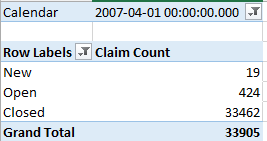
I wonder how many people believe that Tabular DistinctCount outperforms Multidimensional judging by Excel reports alone. In this case, an insurance company reported a performance degradation with Excel reports connected to a multidimensional cube. One report was taking over three minutes to run and it was requesting multiple fields on rows (insured, insured state, insured city, policy number, policy year, underwriter, and a few more) and about a dozen measures, including several distinct count measures, such as claim count, open claim count, and so on. The report would only need subtotals on three of the fields added to the ROWS zone. The cube had about 20 GB a disk footprint so the data size is not the issue here. The real issue is the crappy MDX queries that Excel auto-generates because they are asking for subtotals for all fields added to ROWS, using the following pattern:

NON EMPTY CrossJoin(CrossJoin(CrossJoin(CrossJoin(CrossJoin(CrossJoin(CrossJoin(CrossJoin(

Hierarchize({DrilldownLevel({[Insured].[Insured Name].[All]},,,INCLUDE_CALC_MEMBERS)}),

Hierarchize({DrilldownLevel({[Insured].[Insured City].[All]},,,INCLUDE_CALC_MEMBERS)})),

Hierarchize({DrilldownLevel({[Insured].[Insured State].[All]},,,INCLUDE_CALC_MEMBERS)})),

Hierarchize({DrilldownLevel({[Policy Effective Date].[Year].[All]},,,INCLUDE_CALC_MEMBERS)})),

Hierarchize({DrilldownLevel({[Policy].[Natural Policy Key].[All]},,,INCLUDE_CALC_MEMBERS)})),…

As you can see, the query requests the ALL member of the hierarchy. By contrast, a smarter MDX query generator would request subtotals on the fields that need subtotals only. For example, a rewritten by hand query executes within milliseconds following this pattern:

Hierarchize({DrilldownLevel({[Insured].[Insured Name].[All]},,,INCLUDE_CALC_MEMBERS)}) *

Hierarchize({DrilldownLevel({[Insured].[Insured City].[Insured City].Members},,,INCLUDE_CALC_MEMBERS)})) *

Hierarchize({DrilldownLevel({[Insured].[Insured State].[Insured State].Members},,,INCLUDE_CALC_MEMBERS)}))…

But we can’t change the queries Excel generates and we are at the mercy of the MDX query generator. And, the more fields the report requests, the slower the query would be. DistinctCount measures aggravate the issue further. The problem is that the DC measures cannot be aggregated from caches at deeper levels. Therefore, increasing the number of granularities in the query increases the number of subcubes that are requested from the storage engine, and they’re not going to hit earlier subcubes unless they match at the exact granularity – which is unlikely when the query results are not cached. And at some point, the doubled subcube count will trigger the query degradation (you will see many “Getting data from partition” events in the Profiler). Many of these subcubes are really needed, but some of them are generated for subtotals that Excel doesn’t really need.

I actually logged this issue more than three years ago but the Office team didn’t bother. The original bug was with Power Pivot but the issue was the same. To Microsoft’s credit, the SSAS team introduced an undocumented and unsupported PreferredQueryPatterns setting for both Multidimensional and Tabular, which can be set in msmdsrv.ini (ConfigurationSettings\OLAP\Query\PreferredQueryPatterns). I don’t think it can be set in the connection string. Excel discovers when PreferredQueryPatterns is set to 1 and generates different (drilldown) query pattern instead of the original (crossjoin) pattern. Unfortunately, it looks like more work and testing were done on the Tabular side of things where PreferredQueryPatterns is actually set by default to 1 (although you won’t see it in msmdsrv.ini). I tried a Tabular version of the customer’s cube (only a subset of tables loaded with the biggest table about 50 mil rows fact snapshot and a few distinct count measures) to test with similar Excel queries. With the default configuration (PreferredQueryPatterns=1), Tabular outperformed MD by far (queries take about 3-5 seconds). Initially, I thought that Tabular fares better because of its in-memory nature. Then, I changed PreferredQueryPatterns to 0 on the Tabular instance and reran the Tabular test to send queries with the crossjoin pattern. Much to my surprise, Tabular performed worse than the original MD queries.

PreferredQueryPatterns is 0 by default with Multidimensional due to concerns over possible performance regressions. Indeed, my tests with setting PreferredQueryPatterns to 1 on MD, caused ever-increasing memory utilization until the server ran out of memory so unfortunately it was unusable for this customer. If customer approves, I plan to log a support case. Ideally, the Office team should fix this by auto-generating more efficient MDX queries. If no help on that end, the SSAS team should make PreferredQueryPatterns work with MD. BTW, I was able to optimize somewhat the MD reports by using member properties instead of attributes (from 3 min query execution time went down to 1 min) but that was pretty much the end of the optimization path.

Optimizing Arbitrary Shaped Sets

I’m working on optimizing a fairly large cube (2.5 TB) with some 25 billion rows in the fact table. The customer was complaining about long-running queries. Most queries would specify a time range that was passed to the query filter. For example, if the user wants to see the aggregated data from May 25th 20:00 to June 2nd 19:00, the query WHERE clause would like this:

WHERE

(

{

[Date].[Date].[Date].&[20140527] * [Hour].[Hour].&[20] : [Hour].[Hour].&[23],

[Date].[Date].[Date].&[20140528]:[Date].[Date].[Date].&[20140601] * [Hour].[Hour].&[0] : [Hour].[Hour].&[23],

[Date].[Date].[Date].&[20140602] * [Hour].[Hour].&[0] : [Hour].[Hour].&[19]

}

… additional dimension filters here

)

This an example of using arbitrary-shaped sets which Mosha wrote about here and Thomas Kejser here.

“The resulting union set has interesting shape – it cannot be represented as pure crossjoin of attribute hierarchies. Such sets are nicknamed “arbitrary shaped sets” in Analysis Services, because they represent shapes of arbitrary complexity. Analysis Services in general doesn’t like arbitrary shaped sets, and there are often performance issues when using them, but if the business requirement calls for them – they can be used and will work correctly, although not most efficiently.”

Indeed, the server doesn’t like them and it would happily scan all partitions. In this case, the cube is partitioned by hour and data is kept for 40 days so there are 960 partitions. Although the above query spans 120 hours (partitions), the profiler would show that the server scans all 960 partitions, resulting in enormous amount of data being read. As it turns out, the WHERE clause is not optimized to project the filter on partitions. However, SUBSELECT filters are optimized because most reporting tools, such as Excel and SSRS, use them. The solution was simple: replace the WHERE clause with SUBSELECT to bring the query execution time from minutes to seconds:

FROM

(

SELECT

{

[Date].[Date].[Date].&[20140527] * [Hour].[Hour].&[20] : [Hour].[Hour].&[23],

[Date].[Date].[Date].&[20140528]:[Date].[Date].[Date].&[20140601] * [Hour].[Hour].&[0] : [Hour].[Hour].&[23],

[Date].[Date].[Date].&[20140602] * [Hour].[Hour].&[0] : [Hour].[Hour].&[19]

}

ON 0 FROM [<Cube>]

)

WHERE (… additional dimension filters here)

Partition Bug with Visual Studio

There is a glaring bug with Multidimensional and Visual Studio 2012 and above. When attempting to add a new partition, the Partition Wizard finishes without error but no partition is added. Interestingly, no one has reported this bug more than two years after these Visual Studio editions have shipped. A couple of workarounds exist:

  1. Use SSDT or Visual Studio 2010 to create partitions. You can open your SSAS 2012 project in any Visual Studio edition starting with 2010.
  2. Add the partition either programmatically using AMO or by making changes directly to the *.partitions file.

On the subject of partitions, note that MS has marked the following features deprecated:

  • Remote partitions
  • Remote linked measure groups
  • Linked Dimensions
  • Dimension writeback

These features won’t be terribly missed. I haven’t seen remote partitions being used in real life except in BI certification exams. Linked measure groups also needs linked dimensions, but again, nobody in practice appears to use cross-server linked measure groups. These are cool features “on paper” which could and perhaps should have been popular, but they’ve never caught on enough for various reasons. If you do use them, now it’s time to provide feedback to MS. If you give them a good reason why you need a feature, they will probably reconsider.

Calculating Inception-to-Date Measures

A requirement popped up for calculating an inception-to-date (ITD) measure.

MDX CALCULATED MEMBER

Aggregate(PeriodsToDate ([Date].[Calendar Hierarchy].[(All)]), [Measures].[Sales Amount])

In MDX, ITD is not much different than other time calculations, such as YTD or QTD. We only need to specify that the calculation will be performed over the top-most level of the Date hierarchy whose default name is ([Date].[Calendar Hierarchy].[(All)]. Of course, time calculations should be added to a shell dimension and a scope assignment can be used then in the cube script:

Scope (

[Accounting Date].[Calendar Year].[Calendar Year].Members,

[Accounting Date].[Date].Members ,

[Relative Date].[ITD]

);


this =

Aggregate

(

{[Relative Date].[PTD]} * PeriodsToDate ([Date].[Calendar Hierarchy].[(All)])

);

End
Scope;

DAX MEASURE

=CALCULATE(SUM(‘Reseller Sales'[Sales Amount]), FILTER(ALL(‘Date’), ‘Date'[Date] < MAX(‘Date'[Date])))

In DAX, we pass a table consisting of the dates we need to aggregate over as a second argument of the CALCULATE function. We need to use the ALL function to ignore the row context of the Date table in order to calculate the date range by filtering the date table until the current period. The MAX function is used to get the last date of the current period on the report, e.g. 10/31/2012 if the month is October 2012.

How to Cluster Analysis Services

Some scenarios require a fault-tolerant SSAS installation. In a real-life project, an active-active cluster met this requirement. Instead of installing an active-passive cluster where one node just plays a sitting duck waiting for the active node to fail, with the active-active cluster we had two active nodes to distribute processing and achieve high availability. The first node had the SQL Server database engine hosting the data warehouse database while the second had SSAS. If one of the nodes would fail, its services will fail over to the other.

Configuring a failover cluster requires many steps. Luckily, Microsoft just published a whitepaper “How to Cluster SQL Server Analysis Services” by Allan Hirt (SQL Server MVP) that includes step-by-step instructions of how to configure SSAS (Multidimensional or Tabular) on a Windows Server failover cluster (WSFC). Although not discussed, instead of WSFC, yet another way to achieve high tolerance that gains popularity is to use VM failover capabilities.

5 Tools for Understanding BISM Storage

Recall that the Microsoft BI Semantic Model consists of three flavors: Multidimensional, Tabular, and Power Pivot. The default storage mode of Tabular and Power Pivot is the xVelocity in-memory engine. The default Multidimensional storage is MOLAP. You might want to analyze which objects consume the most storage space. This especially important for Tabular since computer memory is still a scarce resource.

Windows Explorer

The easiest way to get the storage breakdown for Multidimensional and Tabular is to use Windows Explorer and examine the size of the corresponding data folder under the SSAS Data folder, e.g. C:\Program Files\Microsoft SQL Server\MSAS11.TABULAR\OLAP\Data\AdventureWorks Tabular Model SQL 2012.0.db. Unfortunately, Windows Explorer in Windows 7 and 8 doesn’t show the folder size requiring you either to hover on the folder to see its size or to go the folder properties. As a workaround, consider utilities such as HDGraph or Folder Size. Folder Size, for example, pops up a window in Windows Explorer on the side of each folder that has subfolders to show you the folder size. In the case of the AdventureWorks Tabular Model SQL 2012 Tabular database, we can see that Product Inventory table consumes the most space.

041414_0113_5ToolsforUn1

If you drill down the Product Inventory folder and sort by size, you can see the storage breakdown by column.

BISM Server Memory Report

Another way to analyze Tabular and Multidimensional storage in an user-friendly way is to use the BISM Server Memory Report developed by Kasper de Junge (Senior Program Manager at Microsoft).

DMV Views

Behind the scenes, the BISM Server Memory Report uses SSAS DMV Views which expose expose information about local server operations and server health. Specifically, it uses the Discover_object_memory_usage DMV which you can query directly to obtain the same information.

041414_0113_5ToolsforUn2

Power Pivot Macro

If you use Power Pivot, the easiest way to analyze Power Pivot storage in Excel 2013 is to use the Power Pivot macro made available by Kasper de Junge. When you run the macro, it generates Excel pivot report which you can sort by the object memory size. For example, the report below allows us to see the most memory is consumed by CalculatedColumn1 (although xVelocity calculated columns are stored to disk like regular columns, calculated columns are not compressed).

041414_0113_5ToolsforUn3

Power Pivot PowerShell Script

While the above macro relies on Excel 2013 native integration with Power Pivot and only works with Excel 2013, the methodology and PowerShell script developed by Vidas Matelis (SQL Server MVP) works with both Excel 2010 and 2013.

Dynamic Dimensions

Scenario

You need to assign a dimension dynamically to a cube measure group, such as to calculate binning. In the extreme example, you might need to perform fact row level evaluation to determine where the dimension “fits” in. Consider the following example from the insurance industry. An ODS-style Claim table interprets every change to the claim table as a Type 2 change by creating a new row and expiring the previous row of the claim.

Claim_KeyStart_DateEnd_DateClaim_NumberStatus
11/1/20105/1/2010C00001New
25/2/20103/8/2012C00001Open
33/9/201212/31/9999C00001Closed


Options

Given this scenario, you might want to count the number of claims as of any date. You have two options:

  1. Create a Claim Snapshot fact table taken at a daily or monthly interval.
  2. Dynamically associate the Date dimension. In Multidimensional, this will require creating a Claim dimension and a Claim measure group, both bound to the same Claim table. Then, you can use the following script to “associate” the Date dimension (added as a unrelated dimension to the cube) to the Claim measure group:

CREATE MEMBER CURRENTCUBE.[Measures].[ClosingAccountingDate] AS [Date].[Calendar].MemberValue, VISIBLE = 0 ;

Scope

(

(

MeasureGroupMeasures(“Fact Claim”)

{

[Measures].[Start Date],

[Measures].[End Date]

}

),

[Date].[Calendar].Members,

Leaves([Claim])

);

this = iif ([Measures].[ClosingAccountingDate]>=[Measures].[Start Date] and [Measures].[ClosingAccountingDate]<=[Measures].[End Date],

Measures.CurrentMember, null);

End Scope;

End Scope;

To simplify the evaluation, the MemberValue property of all attributes of the Date dimension is bound to the closing date of the period, e.g. 12/31/2014 for year 2014, 3/31/2014 for any day in Q1, and 1/31/2014 for any day in January 2014. The scope assignment includes all measures in the Fact Claim measure group, except the Start Date and End Date measures since we don’t want to overwrite them. It also scopes on all members of the Calendar hierarchy of the Date dimension so that the calculation is performed at any level of the Calendar hierarchy. For example, if the user selects 2014 as a year, the calculation is performed as of 12/31/2014. Moreover, the Leaves([Claim]) scope positions at the measure leaves so we can evaluate any row in the fact table by comparing if the ‘as of’ date falls in the range of Start Date and End Date for that row.

032314_2359_DynamicDime1

Are we happy? We might be but end users might not be so excited. The problem is that this remarkably simple scope assignment can put a remarkable dent in the query performance. For any date, the server has to perform the evaluation for every row in the fact table. With a Claim dimension and a measure group with 500,000 rows, calculating the counts executes relatively fast (within a few seconds). However, running a trend query that requests counts for every day in a quarter might take a minute or so. The larger the claim dimension and the cube subspace that the query requires, the worse the performance will be. The performance is further impacted if you have other calculations on top of the claim counts.

Scope assignments are a very powerful and useful feature of Multidimensional but you shouldn’t abuse them. Keep the scope as narrow of possible to limit the cube space where the calculation is applied. Although it might require ETL effort, materialize whenever you can. For example, although it might result in millions of rows, a snapshot would perform much better with the above scenario. Further, performance can be further enhanced by partitions and aggregations while dynamic granular calculations won’t.

When Dynamic Sets Are Not Dynamic

In my “Optimizing Dimension Data Security” blog, I’ve mentioned that converting static sets to dynamic could reduce the connection initialization time. To my surprise, using Excel to connect to the cube triggered the executing of dynamic sets and end users reported long wait times for the connection to initialize. It turned out that when Excel connects to the cube, it issues DISCOVER statements to query the metadata. One of these statements queries MDSCHEMA_SETS to find out what sets are available in the cube. For some obscure reason, this triggers the actual set evaluation for dynamic sets. If the set is expensive, e.g. touches all partitions, the DISCOVER statement can surely delay the connect time.

It turned out that other users are experiencing the same issue even if security is not applied. Greg Galloway found a workaround and extended the Analysis Services Stored Procedure project with a CurrentCommandIsDiscover method. You can use this method to check if the tool sends a DISCOVER command in your dynamic set definition and short-circuit the set evaluation, like so:

Create Dynamic Set CurrentCube.[Top 25 Selling Products] As

IIf(

ASSP.CurrentCommandIsDiscover(),

Head([Product].[Product].[Product].Members,0),

TopCount

(

[Product].[Product].[Product].Members,

25,

[Measures].[Sales Amount]

)

),

Display_Folder = ‘Sets’;

Passing Large Report Parameters

Scenario: A custom application needs to display a filter dialog to prompt the user to select accounts from a tree consisting of thousands of nodes, such as a tree that organizes the accounts in levels. Once the user makes the selection, the application passes the account list to a report parameter so that the report can show the data for the selected accounts only.

Issue: The filter list could get rather large. Even if the application follows the Excel filtering pattern to include only the parent node if no child nodes are selected, you might end up with a list consisting of hundreds, perhaps even thousands of accounts. However, Reporting Services has limits on the parameter size. When you test the report in the Report Designer, the report parameter is limited to some 32,000 characters. The Report Viewer doesn’t have this limitation so a string-type report parameter can deceptively take the entire list. However, a change was made in SQL 2012 to limit the parameter size during report rendering. Specifically, ParameterInfoCollection.ToUrl throws an exception “The value of parameter ‘param’ is not valid.” when a parameter value exceeds 65,520 characters. That’s because this method calls the .NET System.Uri.EscapeDataString method which has the 65,520 limit. Interestingly, the report query is executed but the error is thrown after the dataset is processed.

Resolution: What if you still need to pass a parameter value whose size exceeds 65,520 characters? Here are some options:

  1. Although not a solution, the easiest approach is prevention, such as to limit the user selection to 65,520 characters.
  2. Another option is to save the report value to a database and pass the table key to the report parameter. Then, the report query can join to the report parameter table. This approach may work well for relational reports but it doesn’t work so well with cube reports because you can’t join the cube to a relational table. You might try to default the report parameter to a database query that brings the report value from the database but you will still get the above error. For cube reports, one option might be to concatenate the report query text with the filter from the database. Another option could be to write an SSAS stored procedure that retrieves the filter from the database and generates an MDX set.
  3. Yet another option is to compress the report parameter. For example, MDX has a rather verbose notation. Instead of passing the member unique name, e.g. [Account].[Account Level 1].&[1000], consider collapsing the level name to |al1|.&[1000] and then expanding it on the report side by replacing the token with the attribute or level unique name. This approach may reduce the parameter list x10 and help you overcome the 65K limit.