Posts

Transactional Reporting with Tabular

Scenario: We had a requirement to replace the existing implementation of transactional reporting over large data volumes. By “transactional reporting” I mean allowing the user to query individual transactions as they’re stored in the fact table. In some cases, this style of reporting requires simply reading data without aggregations. This, of course is what RDBMS are designed for but in our case, requirements call for extending the reporting model with metadata about the item, such as the item barcode, alias, etc., as well as supporting fast aggregation analysis (for trend reports) and data security. In general, when implementing BI solutions, you should always have an analytical layer between the database and presentation layer for the reasons I discussed in the “Why an Analytical Layer?” blog.

Challenges: Because of the in-memory nature of Tabular and more relaxed schema requirements, such as no separation of dimension and fact tables and ability to keep text-based columns in fact tables, we opted for Tabular on top of a data warehouse and star schema. Our initial schema included an Item dimension table (700 million rows) where the item metadata is kept and Transactions table (1.5 billion rows) that stores the item transactions. However, as we found out quickly, this design presented challenges for Tabular:

  1. Excessive processing time – It took very long to process the initial model. By default, SSMS generates a transactional processing batch that supports processing multiple tables in parallel. However, if there is an error during processing the entire transaction is rolled back and you need start from scratch. To avoid this, we tried scripting the batch and changing it to non-transactional (Transaction=’false’). This option preserves the processed partitions but it doesn’t allow tables to be processed in parallel. This is by design to avoid unexpected interactions due to the potential cross-object dependencies in the recalculation chain. Since both the Item and Transactions tables were portioned, the net effect was that the processing was serialized by table and partition when two scripts for processing Item and Transactions are simultaneously executed (partition 1 of Transactions is processed, partition 1 of Item is processed, partition 2 of Transactions is processed, partition 2 of Item is processed, and so on). To make things worse, there is currently a bug with Tabular where the server builds relationships even when Process Data is used as a processing option which further slows down processing.
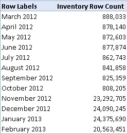
  2. Excessive memory footprint – For some reason, Tabular used a lot of memory with the two table approach. Granted, we had to load the dataset twice (one for Item and a second time for Transactions) but still it should have taken less memory (see the memory footprint in the Solution section). The development server had 80 GB of RAM. We ran out of memory half-way during the full load and ended up with the in-memory model taking 65 GB of RAM.
  3. Excessing query time – This was the worst. When we tried Power View as a reporting tool, each time the Item table was involved in the query, the report took more than a minute to finish. The report filter would return only in a few rows from the Transactions table but when the join was made to the Item table (one the one side of the Item-Transactions relationship), the report performance would degrade significantly. As it turned out, Tabular hasn’t been tuned for such scenarios where queries involve large dimension tables and the filter is applied on the fact table.

Solution: To work around the Tabular limitations, we merged the two datasets by joining the Item and Transactions tables in a SQL view. This approach resolved all issues:

  1. Processing time was reduced x10 because Tabular had to process only one large table.
  2. The memory footprint of the entire database with all the data was reduced to 13.5 GB.
  3. The query times went down to seconds.

The only caveat is that processing would incur a hit because of the join between two large tables but we’d rather spend more time during processing than sacrificing query performance.

At least for now, don’t be confused by the “relational” nature of Tabular. It’s still optimized for queries that request a restricted set of columns and aggregate data. Currently, it’s not optimized for transactional (detail-level) style of reporting that requires many columns and requests data at the lowest level. Microsoft is aware of this and would probably introduce optimizations in time.

In a future blog, I’ll discuss techniques to optimize the query performance with transactional reporting and Tabular. Many thanks to Marius Dumitru (Principal Architect on the SSAS team) for answering my questions.

Improving Tabular Design Experience

When you develop an organizational Tabular model in SSDT, there is always an implicit processing phase for each action you perform, such as renaming columns, creating hierarchies, changing formatting, and so on. This “data-driven” paradigm could be both a blessing and a curse. A blessing, because you always work with data and you don’t have to explicitly process the model to see the effect of the changes. And a curse, because each time you make a change the UI blocks until the change is committed and this can get old pretty soon.

Note: As long as you don’t use the Table Properties dialog or explicitly refresh the data, all changes are done directly in the Tabular database and Tabular doesn’t re-query the data source to refresh the data.

While waiting for Microsoft to make the necessary changes, here are a few tips to improve your Tabular design experience:

  1. In my experience, the size of the dataset doesn’t affect the duration of the “refresh” step. However, I always use a small dataset during development for faster processing. To do this, if you have a large table, partition the table in Tabular and load only one (e.g. the smallest) partition. If you have already loaded all partitions, you can clear all but one with Process Clear. Now, you have a small dataset to work with during development. Once you deploy to the QA or production server, you can process all partitions.
  2. Disable Automatic Calculation – To do this, go to the Model menu and click Calculation Options -> Manual Calculation. Sometimes (depending on model/calculation complexity) disabling automatic calculation in SSDT may help make modeling operations more responsive. To update the calculated columns, once you’re done with the changes, do Model->Calculate Now. Thanks to Marius for this tip.
  3. While the size of the dataset doesn’t affect the refresh duration, the hardware configuration of your development machine does. Suppose you have an underpowered company laptop and a more powerful personal laptop (lots of memory, solid state drive, many cores, etc.) If your company policy allows using your personal laptop, follow these steps to temporarily switch development during the change-intensive part of the design process:
    1. Copy the source from the first laptop to your personal laptop.
    2. Back up and restore the workspace database to your local Analysis Services Tabular instance. If you follow my first tip, the workspace database should be fairly small.
    3. Load the project in SSDS and double-click the Model.bim file to initialize your environment. This will create a second empty workspace database to your local Tabular instance. Close the solution in SSDT. Now, open the Model.bim_<your name>.settings file in Notepad, find the <Database>element and change it to the name of the original workspace database. Open the solution in SSDT. Now you should see the data in your original workspace database.
    4. Perform the design changes. As a comparison, it takes about 5 seconds to commit a change on my laptop vs. 15 seconds on an underpowered laptop.
    5. Once you’re done with the changes, replace Model.bim and Model.bim.layout files on your company’s laptop.

Adding a Set Total

Scenario: You have defined an MDX set in the cube script, such as a set that returns a few months. For the sake of simplicity, we will hardcode the months.

CREATE SET CURRENTCUBE.[12Months] AS

{

[Date].[Month].&[201302].Lag(11):[Date].[Month].&[201302]

};

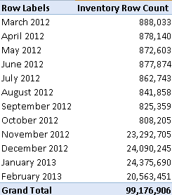
As useful as the set might be, it has an issue. It doesn’t return the total and users might complain about it:

030813_2047_AddingaSetT1

Solution: As a first try, you might attempt to add the [All] member to the set:

CREATE SET CURRENTCUBE.[Last12Months] AS

{

[Date].[Month].&[201302].Lag(11):[Date].[Month].&[201302]

+

[Date].[Month].[All]

};

You’re on the right path. Now, you’ll get the grand total row in Excel but it shows the unrestricted (non-visual total) total instead of the total across set members only. Instead, use the VisualTotals() function:

CREATE DYNAMIC SET CURRENTCUBE.[12Months] AS

{

[Date].[Month].&[201302].Lag(11):[Date].[Month].&[201302]

+

VisualTotals

(

{

[Date].[Month].[All],

[Date].[Month].&[201302].Lag(11):[Date].[Month].&[201302]

}

)

};


030813_2047_AddingaSetT2

Here, the VisualTotals function returns the All member with the total adjusted to set members only. Notice also that I’ve changed the set definition to by dynamic (DYNAMIC keyword) to force re-evaluation of the set.

In a slightly more complicated scenario, what if you want the total to appear as an additional member of the set as opposed to a grand total row. One implementation approach will be to add a dimension calculated member to the Month hierarchy that does the aggregation and then add the new member to the set:

CREATE MEMBER CurrentCube.[Date].[Month].Agg AS Aggregate([Date].[Month].&[201302].Lag(11):[Date].[Month].&[201302])

CREATE SET CURRENTCUBE.[12Months] AS

{

[Date].[Month].&[201302].Lag(11):[Date].[Month].&[201302]

+

[Date].[Month].Agg

};


CU2 for SQL Server 2012 SP1

Microsoft released a while back a cumulative update 2 for SQL Server 2012 SP1. Besides other things, it includes a fix for the “wide” MDX query performance degradation issue with Analysis Services that I previously reported.

  • Knowledge base for the performance issue
  • Knowledge base with SP1 CU2 download link

Performance Degradation with the Aggregate Function and Unrelated Dimensions

I ran into a severe performance issue with the Aggregate function and unrelated dimensions which I reported on connect. In this context, an unrelated dimension is a dimension that doesn’t join any measure group in the cube. Why have unrelated dimensions? My preferred way to implement time calculations is use a regular dimension that is added to the cube but not related to any measure groups. Then, I use scope assignments to overwrite the time calculations, e.g. for YTD, MTD, etc. For example, the scope assignment for YTD might look like:

Scope (

[Relative Date].[YTD]

);


this =


Aggregate

(

{[Relative Date].[Current Period]} * PeriodsToDate([Date].[Fiscal].[Fiscal Year], [Date].[Fiscal].CurrentMember)

);

End Scope;

Notice the use of the Aggregate function which when executed maps to the default aggregation function of the underlying measure. For some reason with SQL Server 2012, a query that uses the Relative Date dimension experiences a significant performance hit. Replacing Aggregate with Sum fixes the issue, assuming you can sum up the affected measure to produce the time calculations.

DAXMD Goes Public!

Microsoft announced yesterday the availability of the Community Technology Preview (CTP) of Microsoft SQL Server 2012 With Power View for Multidimensional Models (aka DAXMD). As a participant of the CTP program and I’m very excited about this enhancement. Now customers can leverage their investment in OLAP and empower business users to author Power View ad-hoc reports and dashboards from Analysis Services cubes. Previously, Power View supported only PowerPivot workbooks or Analysis Services Tabular models as data sources. I’m not going to repeat what T.K. Anand said in the announcement. Instead, I want to emphasize a few key points:

  1. This CTP applies only to the SharePoint-version of Power View. Excel 2013 customers need to wait for another release vehicle to be able to connect Power View in Excel 2013 to cubes.
  2. You’ll need to upgrade both the SharePoint server and SSAS server because enhancements were made in both Power View and SSAS.
  3. Although not supported, I successfully tested that you can install the CTP on top of SQL Server 2012 SP1.
  4. The CTP will not be upgradable to RTM.
  5. It’s not known at this point when and how the RTM bits will ship.
  6. DAXMD doesn’t translate DAX queries to MDX. Instead, the DAX queries are handled natively on the server and performance is awesome!

Kudos to the SSAS and SSRS teams for listening to customers and working together on this feature!

Book Review “Microsoft SQL Server 2012 Analysis Services – The BISM Tabular Model”

I’ve recently had the pleasure to read the book “Microsoft SQL Server 2012 Analysis Services – The BISM Tabular Model” by Marco Russo, Alberto Ferrari, and Chris Webb. The authors don’t need an introduction and their names should be familiar to any BI practitioner. They are all well-known experts and fellow SQL Server MVPs who got together again to write another bestseller after their previous work “Expert Cube Development with Microsoft SQL Server 2008 Analysis Services”. The latest book was published about five months after my book “Applied Microsoft SQL Server 2012 Analysis Services: Tabular Modeling”. Although both books are on the same topic, we didn’t exchange notes when starting on the book projects. In fact, I was well into writing mine when I learned on the SSAS insider’s discussion list about the trio’s new project. Naturally, you might think that the books compete with each other but after reading Microsoft SQL Server 2012 Analysis Services – The BISM Tabular Model” I agree with Marco and Chris that the books actually complement each other pretty well.

A central theme of my book is the continuum of Self-service, Team, and Organizational BI. I felt that it is very important to show how Tabular addresses the needs of both business users and BI pros. Indeed, the Tabular journey can start very unassuming, perhaps with a business user creating a simple personal model, gains popularity and evolves to a deployed model shared by teammates, and finally to a corporate model that is provisioned and sanctioned by IT. Because of this, the first part of the book covers PowerPivot for Excel, the second covers PowerPivot for SharePoint, and the third part covers Analysis Services Tabular. Since my book naturally targets different reader audiences (business users, power BI users, and BI pros), I felt that it was imperative to lower the learning curve as much as possible, such as providing step-by-step instructions for the exercises and video tutorials. Writing a book that targets such a broad base is not easy. To make sure that the book will be well accepted, I had readers who represented each of these groups review the manuscript and provide feedback.

On the other hand, Microsoft SQL Server 2012 Analysis Services – The BISM Tabular Model focuses on the professional side of Analysis Services Tabular and targets mainly BI pros. More than half of the book is devoted on DAX and you’ll be hard pressed to find a better coverage on this topic (a note to myself that DAX deserves more attention if I ever write a revision). Besides DAX, Microsoft SQL Server 2012 Analysis Services – The BISM Tabular Model covers equally well other aspects of Tabular and the author’s real life experience shows through. My favorite chapters are Chapter 11 “Data Modeling in Tabular” and Chapter 12 “Using Advanced Tabular Relationships”.

All in all, any serious BI pro willing to learn Tabular should have this book on the shelf… I hope next to mine.

Fix for “Wide” MDX Query Performance Degradation

We ran into a situation where a wide MDX query requesting many regular and semi-additive measures side by side can degrade the Analysis Services server performance. As I explained in this connect bug report, the customer had a Reporting Services report that includes many measures (close to a hundred). Users insisted on having this report to be able to export all results in Excel and pivot on them. Of course, one of the advantages of having a cube is to make this exact requirement unnecessary but old habits die hard. We’ve noticed that when the report includes 75 measures from a single measure group, the query executes within 20 seconds. However, when adding more measures from the same measure group, the query performance degrades to minutes. The measures are either regular (persisted) measures or simple calculated member wrappers and don’t use any intensive formulas or scope assignments. The important point is that the query requests both additive and semi-additive measures (in our case the semi-additive measures use the LastChild function).

Microsoft determined that the performance degradation occurs when the number of overlapping calculations for a part of the cube space exceeds a threshold causing the server to switch from block mode to cell by cell evaluation for the affected query space. Microsoft was quick to provide us with a private fix that addresses the issue by distinguishing when the overlapping calculations are due to semi-additive measures vs. scope assignments in the cube script or query scope calculations (the reason the original limit was present). It will also allow the administrator to configure the threshold by adjusting the MaxCoverItemOverlapCount setting in msmdsrv.ini file although raising this number too high could result in negative performance on some cases where the cell by cell evaluation of highly complex calculations is faster than the block evaluation method. The official fix will be included in CU4 for SQL Server 2012 expected in mid-October 2012. I’m not sure about if the fix will make it to the older versions of SQL Server.

Localizing Reports in SharePoint

In a current project, international users indicated that they prefer dates and numbers to be formatted using their regional settings. Localization is a big and complicated topic and we’ve been fortunate that the scope was limited to just number and date formatting … or, at least so far.

Localizing reports on a report server running in native mode is easy. You just need to use culture –neutral format strings, e.g. C for currency of P for percentage, and set the report-level Language property to =User!Language. However, this is not enough for reports running in a SharePoint integrated mode. SharePoint requires installing language packs as follows:

  1. For each language you plan to support, download the corresponding language pack. For example, to download the German language page, change the drop-down to German and download the pack.
  2. Log in a SharePoint Farm Administrator and install the language pack. At the end of the setup process, leave the checkbox to start the wizard in order to run the wizard to reconfigure the farm.
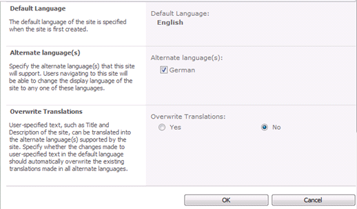
  3. Once the wizard is done, go to the site that you want to localize, click Site Actions -> Site Settings, and then click the Language Settings link under Site Administration.
  4. Check all languages that will be supported on the site.

    072312_2000_LocalizingR1

  5. To avoid “The LocaleIdentifier property is not overwritable and cannot be assigned a new value” error (more than likely a bug) when an international user requests a report connected to an Analysis Services cube, change the connection string of the SSAS data sources to pin it to the locale identifier of the server by appending the following setting, as Kasper De Jonge mentions in his blog:
    Locale Identifier=1033
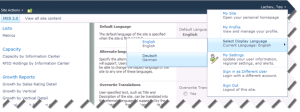
  6. Instruct your users to personalize the display language by expanding the name drop-down and selecting a display language:

    072312_2000_LocalizingR2

Once this is done, the users will see the SharePoint menus translated, and dates and numbers on the reports formatted using the selected display language.