Posts

Offsetting Week Start Day

Scenario: You have a date dimension table and typical date-related columns, such as DayOfWeek, WeekEndDate, etc. In US, weeks start on Sunday and end on Saturday (ISO weeks on the other hand start on Monday and end on Sunday). You have a requirement to overwrite the week start and end days for a Power Pivot, Tabular, or MD model. For example, while the Date table defines the week start day on Sunday, you might need to overwrite it to start on Monday.

Solution: I typically derive as many of the date calculations in a SQL view on top of the Date table instead of saving the results in the table itself. For example, the WeekOfYear calculation might look like this:

DATEPART(WEEK, [Date]) [WeekOfYear]

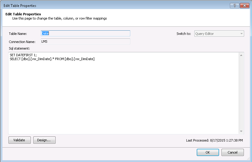
If you have date calculations like this, instead of changing all week-related calculations to reflect the desired week start day, the easiest way to offset the week day is to use the T-SQL SET DATEFIRST statement preceding the actual SELECT statement. The following example taken from Power Pivot/Tabular overwrites the first day of the week to start on Monday.

BISM Drillthrough Capabilities

All the three BISM flavors (Multidimensional, Tabular, and Power Pivot) supports default drillthrough to allow the end user to see the level of details behind an aggregated measure by just double-clicking the cell. However, the implementation details differ. Multidimensional supports default drillthrough on regular measures only, that is, measures that bind to columns in fact tables. Multidimensional doesn’t support drillthrough on calculated measures, even if these measures are simple tuples, such as ([Measures].[Sales Amount], [Product].[Product Category].[Some Category]).

On the other hand, Power Pivot and Tabular don’t have the concept of regular measures and they support only calculated measures. Even if the user drags a column to the Values zone on a pivot or Power View report, the tool creates an implicit measure with a DAX formula behind the scenes, such as =SUM(ResellerSales[Sales Amount]). Because of this, Power Pivot and Tabular appears to allow drillthrough on any measure. However, the drillthough action only picks the filter context. It does not parse the calculated measure. So, if you have an explicit measure with a DAX formula that filters the results, such as =CALCULATE( SUM( ResellerSales[Sales Amount] , FILTER(SalesTerritory, SalesTerritory[Country] = “USA” ) ), the drillthrough action won’t return the rows where country=’USA’. Instead, it will return the rows from the ‘home’ table within the default context inferred by rows, columns, and filters on the report.

While we are on the subject of drillthrough, Multidimensional allows the modeler to specify custom actions, such as an action that runs an SSRS report or opens a web page. As it stands, Power Pivot and Tabular don’t provide UI for custom actions although the drillthrough functionality is there. As a workaround, you can use the BIDS Helper Tabular Actions Editor feature to implement custom drillthrough actions.

Presenting at SQL Saturday Atlanta

The next Atlanta SQL Saturday will be on May 3rd. I’m doing a “Deep Dive into the Microsoft BI Semantic Model (BISM)” pre-conference session on May 2nd. You can register using this link. The organizers set up a promotion code for $10 off registration, good for the first 10 users – the code is “AtlantaBI”.

Teo Lachev: Deep Dive into the Microsoft BI Semantic Model (BISM)

SQL Saturday #285 – Atlanta

Friday, May 2, 2014 from 9:00 AM to 4:30 PM (EDT)

“The chances are that your organization has a centralized data repository, such as ODS or a data warehouse, but you might not use it to the fullest. Join this insightful full-day event to understand the importance of having a semantic layer that bridges users and data. In the Microsoft BI world, BISM consists of Power Pivot, Tabular, and Multidimensional.

We’ll start by comparing these technologies to understand their usage scenarios, strengths and shortcomings. Next, we’ll put our business user’s hats and see how Power Pivot and the rest of the Microsoft self-service BI stack helps you integrate data from multiple data sources, implement self-service BI data models with Excel to ideate and promote divergent thinking.

Next, we will follow the BI continuum and see how to share these models and reports with your teammates by deploying them to SharePoint. Business intelligence professionals will discover how to build scalable and secure organizational solutions powered by Tabular and Multidimensional that deliver supreme performance with large data volumes and promote a single version of the truth.”

I submitted also a session proposal “Real-time BI with StreamInsight” for Saturday. It’ll be a busy SQL Saturday for me.

020114_0320_Presentinga1

Handling Dates in BISM Tabular

[View:https://prologika.com/CS/cfs-file.ashx/__key/CommunityServer.Blogs.Components.WeblogFiles/blog/2308.AdventureWorks.zip:550:0]If you have experience with multidimensional cubes, you know that most cubes have a Date dimension grained at a day level. If the fact table has multiple date keys, you can join the Date dimension multiple times to the measure group so the Date dimension can play multiple roles (a role-playing dimension), such as OrderDate, ShipDate, and DueDate. If you use Excel pivot reports connected to the cube, to get support for dates you need to make the following changes as explained in Designing SQL Server 2005 Analysis Services Cubes for Excel 2007 PivotTables:

  1. Set the Type property of the Date dimension to Time. This is also required for MDX time-related functions, such as YTD.
  2. Set the ValueColumn column of the Date key to a column of date data type.

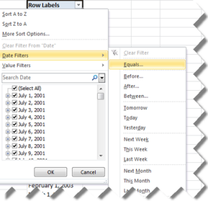
Once this is done, Excel “understands” the date semantics and treats dates as dates when you sort and filter on any field from the Date dimension. It also shows a nice menu for time calculations (relative dates).

103011_2341_HandlingDat1

But what if another dimension has a date attribute, such as the customer’s birth date? Unfortunately, Excel won’t recognize this field as of date type and it will treat as text. Not good, but these are the limitations of Excel OLAP pivot reports.

How does BISM Tabular change things as far handling dates? Starting with SQL Server 2012 and PowerPivot version 2, you can mark a table as a Date table. In the process of doing so, you need to specify a unique identifier. Once this is done, you get the same support for dates with Excel pivot reports because they are actually OLAP pivot reports that see BISM Tabular models as cubes. Specifically, Excel will treat only fields from the Date table as dates. Take for example the following model (attached in the blog):

103011_2341_HandlingDat2

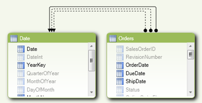
The Orders table has three date fields (OrderDate, DueDate, and ShipDate). In SQL Server 2012, BISM Tabular and PowerPivot support multiple joins between tables, as Kasper de Jonge explains in his PowerPivot Denali: Working with multiple relationships between two tables blog. Well, kind of, because only one join can be active (the one in the solid line). The other dotted relationships can be used for DAX calculations, such as SalesAmountByDueDate, SalesAmountByShipDate, etc. In other words, BISM Tabular doesn’t support true role-playing tables and you won’t get automatically DueDate and ShipDate instances of the Date table. You can import the Date table multiple times but only one table can be marked as a Date table. However, Power View (code-named Crescent) is designed from ground up to support natively BISM Tabular models. Consequently, the Excel date limitations disappear, as shown in the table below.

Date FeaturesExcelPower View
Date typesOnly in Date tableAll tables
Relative DatesOnly in Date tableN/A


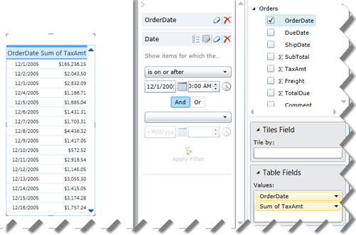
Power View treats any Date field as a date. For example, this Power View report shows the OrderDate and TaxAmt fields from the Order table. The OrderDate field is of date data type. As you can see, I can filter on dates after a given date and Power View shows the correct results. Unfortunately, Power View doesn’t support relative dates as Excel does so you must define DAX time calculations.

103011_2341_HandlingDat3

In short, here are some recommendations to get the most of dates:

  1. If you need to support multiple dates, leave the columns as a of date data type. Don’t use integer keys or smart keys, which are a common practice in data warehousing, to join to the Date table.
  2. Have a Date table that joins to the date that is mostly commonly used so users can aggregate by quarters, years, etc. Make sure that the date columns in the other tables don’t include times because you won’t be able to join 10/19/2011 8:40 PM to 10/19/2011. If you need to have the same support for the other dates, reimport the Date table multiple times.
  3. Consider creating inactive relationships for the other dates to be able to implement DAX calculations.
  4. Use Power View for reporting. Besides better handling of dates, Power View will give you better performance with transactional reporting, as I explained in my Transactional Reporting with BISM Tabular blog.

BTW, speaking of dates and BISM Tabular, Boyan Penev (MVP SQL Server) has implemented a nice Date Stream feed on Azure Data Market. If you decide to consume the feed, you would notice that the DateKey column is returned as ISO8601 date (such as 2011-10-29T00:00:00. Unfortunately, Excel doesn’t recognize the ISO8601 format. You might think that you can around this predicament by creating a calculated column that removes the time portion but you can use a calculated column as a unique identifier in the Date table. As a workaround, save the feed as a file and strip out the time portion so you can set the data type to Date.

BISM Tabular Dynamic Data Security Over Bridge Table

About four years ago, in my article Protect UDM with Dimension Data Security, I introduced an approach to secure dimension data in multidimensional cubes by using a factless bridge table. Since then, many BI practitioners have favored this approach because of its simplicity, reusability (transactional reports can join to the security table), and performance. Now that organizational tabular projects support data security, I wanted to try it with BISM Tabular. As it turned out, the factless bridge table approach worked out just fine.

Suppose that you’ve build a tabular project on top of the Adventure Works DW database and the SecurityResellerFilter table is the bridge table that stores the resellers that an employee is authorized to view. As shown in the diagram, SecurityResellerFilter has two relationships SecurityResellerFilter[EmployeeKey] and Employee[EmployeeKey] and SecurityResellerFilter[ResellerKey] and Employee[ResellerKey]. You’d probably want to hide the SecurityResellerFilter table so the end users can’t browse it.

092811_1402_BISMTabular1

Given this model, implementing a dynamic data security over SecurityResellerFilter requires setting up a new role (click the Roles button in the Analysis Services toolbar) that uses a row filter.

092811_1402_BISMTabular2

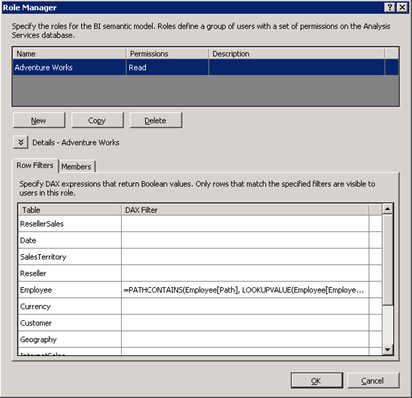
A row filter defines a filter expression that evaluates which rows the role is allowed to see. To set up a row filter in the Role Manager, enter a DAX expression next to the table name. The DAX expression must be a Boolean expression that returns TRUE or FALSE. The Adventure Works role uses the following DAX expression for the row filter on the Employee table:

=CONTAINS(RELATEDTABLE(SecurityResellerFilter), SecurityResellerFilter[EmployeeKey], LOOKUPVALUE(Employee[EmployeeKey], Employee[LoginID], USERNAME()))

The LOOKUPVALUE function is used to obtain the employee key associated with employee’s Windows login which we get from the Username function. Because the row filter is set on the Reseller table, for each reseller the CONTAINS function attempts to find a match for the combination of the reseller key and the employee key. Notice the user of the RELATEDTABLE function to pass the current reseller. The net effect is that the CONTAINS function returns TRUE if there is a row in the SecurityResellerFilter table that matches the ResellerKey and EmployeeKey combination.

You can use the Analyze in Excel feature (click the Analyze in Excel button in the Analysis Services toolbar) to test the security changes. To verify that the user has access only to resellers the user is authorized to see, add the ResellerName field from the Reseller table in the Column Labels zone.

092811_1402_BISMTabular3


The report should show on columns only the resellers that are associated with the interactive user in the SecurityResellerFilter table.

Cube vs. VertiPaq Query Performance

This is a big topic and frankly it’s too ambitious on my part to tackle it. Assuming equivalent multidimensional (BISM Multidimensional) and tabular (BISM Tabular) models, I was curious how a multidimensional cube fares against VertiPaq in terms of performance. To be fair to VertiPaq, I decided to use native DAX queries. As you’ve probably heard, BISM Tabular in SQL Denali will include a variant of DAX to query tabular models deployed to SharePoint and SSAS running in VertiPaq mode. Chris Webb has a good writeup about DAX queries here. The DAX EVALUATE construct allows external clients to query tabular models using native DAX syntax instead of MDX. Since BISM Tabular speaks DAX, DAX queries are likely to be more efficient and give you better performance when querying tabular models. At this point, only Crescent generates native DAX queries. The DAX query syntax is:

DEFINE

MEASURE Table1 [measure1] = <DAX_Expression>

MEASURE Table2 [measure2] = <DAX_Expression>

EVALUATE <DAX Table Expression>

ORDER BY

    <DAX_Expression> [ASC | DESC]

    <DAX_Expression> [ASC | DESC]

START AT

    Value_or_Parameter, Value_or_Parameter, …

To have a more sizable dataset, I used the Contoso cube for my tests. I created a BISM Tabular model and imported the Contoso data. Since you probably don’t have Contoso, I provide queries that target the Adventure Works cube. I’ve started with the following unoptimized MDX query which calculates the average sales amount by date across products whose daily sales exceed the daily sales for the same date in the previous month:

WITH


MEMBER [Measures].SlowAvg AS


Avg

(


Filter

(

[Product].[Product].[Product].MEMBERS

,[Measures].[Sales Amount] > ([Measures].[Sales Amount], ParallelPeriod([Date].[Calendar].[Month]))

)

,[Measures].[Sales Amount]

)

SELECT

[Measures].SlowAvg ON 0,

[Date].[Calendar].[Date].Members
ON 1

FROM [Adventure Works];

Then, I optimized the query to take advantage of block computation mode, as follows:

WITH


MEMBER diff as
iif ([Measures].[Sales Amount] > ([Measures].[Sales Amount], ParallelPeriod([Date].[Calendar].[Month])), [Measures].[Sales Amount], null)


MEMBER [Measures].SlowAvg AS


Avg

(

[Product].[Product].[Product].MEMBERS, diff

)

SELECT

[Measures].SlowAvg ON 0,

[Date].[Calendar].[Date].Members
ON 1

FROM [Adventure Works];

Finally, my equivalent DAX query that used to measure performance was:

define measure FactResellerSales[TotalSales] = Sum([SalesAmount])

measure FactResellerSales[TotalSales – LastYear] = [TotalSales](SamePeriodLastYear(DimDate[FullDateAlternateKey]), All(DimDate))

measure FactResellerSales[AverageSales] = AverageX(Filter(Values(DimProduct[ProductKey]), [TotalSales] > [TotalSales – LastYear]), [TotalSales])

evaluate addcolumns(filter(values(DimDate[DateKey]), not isblank([AverageSales])), “AverageSalesAmount”, [AverageSales])

order by [DateKey]

And, the findings from the tests:

1.       MDX query un-optimized (cell calculation model) both on cold cache and executed second time – 33 sec

2.       MDX query optimized (block computation mode) on cold cache – 4.8 sec

3.       MDX query optimized (block computation mode) executed second time – 0.7 sec

4.       DAX query both on cold cache and executed second time – 6.4 sec

Here are some take-home notes:

  1. The fact that VertiPaq is an in-memory database doesn’t mean that it will perform much better than a multidimensional cube. The formula engine of BISM Multdimensional does cache query results in memory. So does the Windows OS. In fact, the more the cube is used, the higher the chances that its data will end up in memory.
  2. VertiPaq might give you good performance without special tuning. All DAX calculations run in a block computation mode.
  3. Optimized MDX queries might outperform VertiPaq especially if results are cached.
  4. DAX queries are never cached which explains why DAX queries perform the same when executed subsequently.

The fact that VertiPaq gives you a head start doesn’t mean that you cannot write inefficient DAX queries. For example, the following DAX measure definition returns the same results but it’s twice as slow.

measure FactResellerSales[AverageSales] = AverageX(Filter(AddColumns(Values(DimProduct[ProductKey]), “x”, [TotalSales]), [x] > [TotalSales – LastYear]), [x])

Again, this is an isolated test case and your mileage might vary greatly depending on queries, data volumes, hardware, etc. But I hope you could use it as a starting point to run your own tests while waiting for a VertiPaq performance guide.
Business Intelligence Semantic Model – TechEd Redux

While I’ve been busy at TechEd talking to BI enthusiasts, professionals and wannabes and delivering sessions, the news is out about the new BI roadmap and BISM positioning. See:

  • T.K. Anand blog
  • T.K. Anand & Ashvini Sharma recorded session What’s New in Microsoft SQL Server Code-Named “Denali” for SQL Server Analysis Services and PowerPivot”?
  • Sean Boon, Carolyn Chao, and Sabrena McBride recorded session Abundantly “Crescent”: Demos Galore
  • Julie Strauss’ recorded session The Next Generation Design Tools for Analysis Services
  • And the feedback from the community insiders, including Chris Webb’s Good News on the Future of Analysis Services blog, Marco Russo’s Microsoft Updates its BI Roadmap blog, and Boyan Penev’s SSAS to BISM – Recent Developments blog.

So, I won’t repeat what’s been already said. Instead, I’ll attempt to summarize my thoughts about the new BI developments and give you some take-home points to help you plan future BI work.

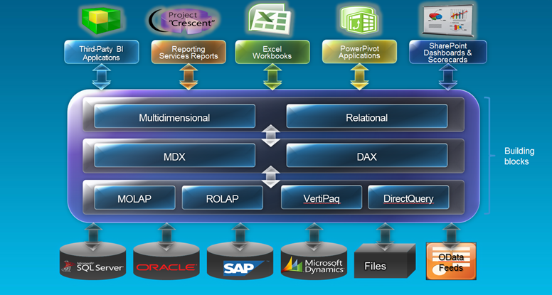
  • I spent many hours with the SSAS and SSRS product groups at TechEd. I liked what I saw. I saw the SSRS and SSAS teams working together. I saw the impressive visualization capabilities of the sleek Crescent tool which will give the competition a run for their money. And I saw the future of Analysis Services and Microsoft BI platform – the new BISM model that is positioned to become what UDM promised to be.
  • BISM is now the unifying name for both the Multidimensional (OLAP) and Tabular or Relational (in-memory) models. Both models will support MDX and DAX query options. Consequently, Excel can see a tabular model as a cube and query it with MDX, while Crescent will be able to see an OLAP cube as a tabular model and send DAX queries to it. This is awesome news that warrants retreating the Ugly part from my blog Business Intelligence Semantic Model – The Good, The Bad, and the Ugly. Kudos to Microsoft for listening to the community and kudos to MVPs for providing relentless feedback!
  • Make no mistake though. Although the external interfaces are the same and there is a significant feature overlap, in Denali the two models will not compatible with each other and no migration path will be provided, e.g. OLAP to Tabular or vice versa. An analogy might be helpful here. Think of Microsoft Access and SQL Server relational databases. Both of them are databases, both support SQL, and both have similar features (tables, relationships, etc.). We could use the label “Relational Database Model” as a unifying name for both databases although each path leads to a completely different model. So, why we are implying a unification here? Think of BISM as a prediction of the future. In time, Tabular may “borrow” OLAP features, such as MDX scripts and OLAP may get Tabular’s elements, such as in-memory partitions. Thus, the divide between the models might blur to a point where the two paths converge into a single model.
  • The most important thing to remember is that the Tabular model is not a replacement for OLAP cubes. Anybody and I repeat anybody, who claims the opposite should be brought to justice and tried in the BI Court. T.K. Anand from the Microsoft SSAS team has actually a faster procedure of strangling that person with his bare hands. You should see Tabular as completing and not competing technology to OLAP, a technology that opens interesting possibilities that were not previously possible with OLAP alone.
  • Regardless of naming and marketing, the question in everybody’s mind moving to Denali would be which path and model to choose for new projects. And, here is my simplified personal plan based on the type of the BI project at hand:

    Self-service BI – This is a no-brainer – PowerPivot and Excel. If you want to let business users analyze data on their own, look no further than Excel.

    Team BI – How do business users share PowerPivot models with other users? SharePoint and PowerPivot of course. Another no-brainer.

    Corporate BI – This is where things get trickier. Let’s go through a few scenarios:

  1. If you’ve started on the PowerPivot path but have exceeded the PowerPivot capabilities, e.g. you need more data (above 2GB) or row-level security, then a PowerPivot model migrated to Analysis Services running in a VertiPaq mode will be a logical choice. This will give you a nice continuum of self-service BI – Corporate BI on a single platform.
  2. If all you need is a simple model that wraps a layer over a raw database or warehouse for reporting & analytics and you don’t have experience with OLAP, consider a tabular model and DAX because of its lower learning curve and less rigid data schema requirements. The issue I have with the “simple” model is that based on my experience many projects start simple but grow exponentially in complexity over time. A many-to-many relationship may creep in, as well as time calculations, currency conversion, etc. So, be careful here, evaluate requirements (if you have them) and take your time to weigh out features and prototype because switching from one model to another will require a complete rewrite. Continuing the Relational Database analogy above, it will feel like moving from Access to SQL Server and you won’t have a wizard. Denali Tabular won’t support OLAP features that we grew to love, such as declarative parent-child and many-to-many relationships (it does support them via DAX calculations but you’ll end up with a calculated measure for each numeric column as in the SSAS 2000 days), scope assignments for implementing time calculations, allocations and currency conversion, Excel what-if analysis, default members, named sets, and others. Although easy to start with, DAX calculations can become complex to a point where you might wonder what you are really saving by switching from MDX to DAX if you are after avoiding the MDX learning curve.
  3. Enterprise-wide BI and Data Warehousing – Here, I’d stick with multidimensional OLAP cubes for now. I won’t bet complex and high-visibility projects on Tabular, at least not for Denali. First, more than likely such projects will require the features I mentioned above. Second, I’d give Tabular some time to marinate in the corporate space. Finally, in Denali only Crescent will support Tabular natively via DAX. In comparison, there are many clients that are optimized to support MDX and OLAP cubes.

I’d like to indulge myself and think that one day, I hope in not so distant future, BISM will evolve to become a true single model that delivers on the UDM promise and combines the best of OLAP and Tabular. Then, we would be able to pick and mix features from both OLAP and in-memory paths, e.g. an in-memory storage with MDX calculations, and use the best technology for the task at hand. Until then, we will have to choose between the multidimensional and tabular paths.

052011_0128_BusinessInt1

Estimating Data Compression

Now that the age of in-memory databases has dawned on us, I’ve been experimenting with different aspects of VertiPaq and I find its technology fascinating. It’s safe to say that VertiPaq will propel Microsoft Business Intelligence for years to come with all of its three flavors: PowerPivot (self-service BI), Business Intelligence Semantic Model (corporate BI), and data warehousing (column-based stored indexes). Unlike Analysis Services MOLAP, which compresses data by rows, VertiPaq compresses data by columns.

Column-based compression fits business intelligence like a glove because data is typically analyzed by columns. And, the lower the data cardinality (that is the more repeating values a column has), the higher its compression rate will be. Since most columns used for analytics fit this category, you could expect 10-15 times data compression. Consequently, a half terabyte database could potentially fit into 80 GB of memory. Notice that I account for more memory because when data is brought from disk into memory, additional space is needed to accommodate index tables and other structures. So, how is this not cool? Moving to BISM, all of your data could fit into memory so you could get a head start in performance just by having a superfast storage medium!

Continuing this line of thought, I decided to take the Contoso Retail DW database and a real-life data warehouse for a spin to see how VertiPaq compresses them. I used the excellent PowerShell script that Vidas Matelis developed. Since fact tables typically contribute to 95% of the data warehouse storage space, I focused on only one fact table from both databases. To measure the VertiPaq compression, I loaded the fact tables into PowerPivot and run the script to obtain their storage space.

MOLAP

VertiPaq

Contoso (FactSales)

129 MB

35 MB

DW (20 mil fact table)

810 MB

792 MB

As you can see, the Contoso VertiPaq results are very impressive. But what happened with the real-life DW? How could VertiPaq be only marginally better than MOLAP? To analyze this further, I used the script ability to get a column compression breakdown and I’ve noticed that the following top two columns occupy the most space:

TRANS_DTLS_KEY: 400 MB (primary key)

LOG_ID: 268 MB (transaction identifier)

Both of these columns are high-cardinality columns. I used these columns in a cube drillthrough action to get the transaction details behind a cell. Subsequently, I added them to PowerPivot so I could compare the same data structures. Currently, PowerPivot doesn’t support drillthrough so adding these columns to PowerPivot is probably not needed in real life. It will be interesting to see how BISM will implement drillthrough. One thing is sure: it makes sense to leave high-cardinality attributes out of VertiPaq and possibly use report actions (if supported) to report on details.

VertiPaq Column Store

In SQL 11, the VertiPaq column store that will power the new Business intelligence Semantic Model (BISM) will be delivered in three ways:

1. PowerPivot – in-process DLL with Excel 2010.

2. A second storage mode of Analysis Services that you will get by installing SSAS in VertiPaq mode.

3. A new column stored index in the SQL RDBMS.

The third option picked up my interest. I wanted to know if a custom application will be able to take advantage of these indexes outside VertiPaq. For example, this could be useful for standard reports that query directly the database. It turns out that this will be possible. The following paper discusses columnstore in more details. In a nutshell, SQL 11 will run the VertiPaq engine in-process. Here are some highlights of the VertiPaq columnstore:

  • You create an index on a table.
  • You cannot update the table after the index is created. Not a big limitation since a data warehouse is typically loaded on a schedule so the index can be dropped and rebuilt at the end of the ETL process.
  • The relational engine scans the entire table and loads it into memory in a Vertipaq store. As you could imagine, the more RAM the better.
  • Query performance will be great but probably slower than VertiPaq in SSAS.
  • Creation of this index isn’t cheap, but the query performance gains should justify using it in common DW scenarios.
  • From performance standpoint, it will be best to load data in VertiPaq (SSAS store) instead of using column store.