Warning: This blog contains old tricks of an old dog.
Scenario: Suppose you have a large table in SQL Server, e.g. hundreds of millions or even a billion rows. DML operations (SELECT, INSERT, UPDATE, DELETE) take long time. How do you speed them up? Do you split the large table into multiple tables? Or, do you ask for better hardware? Or, do you start looking for a new job with less data?
Solution: It’s nothing new but I see clients struggle with this all the time because they don’t know any better.
The solution is to partition the table and use partition switching that SQL Server has supported since time immemorial.
Cathrine Wilhelmsen has a great step-by-step blog covering different scenarios, but the process goes like this:
Configure page compression for the large table (see benefits here).
Partition the large table, such as by month.
Create a not-partitioned staging table that has the same indexes and compression as the large table.
Find the corresponding partition in the large table that will require DML, such as by using this script.
If the data requires updates, switch out the affected partition to the staging table. Perform updates. For full loads where rows will be only inserted, you don’t have to switch out the partition (see the second scenario in Cathrine’s blog).
Switch in the staging table into the corresponding partition of the large table. This should take a few seconds.
As a bonus, the SQL Server query processor could eliminate partitions for SELECTs, thus improving the query performance.
https://prologika.com/wp-content/uploads/2016/01/logo.png00Prologika - Teo Lachevhttps://prologika.com/wp-content/uploads/2016/01/logo.pngPrologika - Teo Lachev2023-03-24 12:23:162023-03-24 12:23:16Working with Large Tables in SQL Server
BI implementation shortcuts are tempting and disguise themselves as cost-effective. True, you can slap a Power BI dataset on top of your data (the cornerstone of self-service BI), but most BI implementations will greatly benefit from a datamart, irrespective of the propaganda of self-service BI vendors. I explain the benefits of datamarts vs Power BI datasets directly on data sources in my blog “Datasets vs. Datamarts”. This newsletter discusses a newly released Power BI feature that attempts to simplify the implementation of datamarts by business users.
Understanding Datamarts
Let’s define a datamart as a centralized repository for hosting clean and trusted data that is typically organized in a star schema, i.e. as a set of fact tables and dimension (lookup) tables. BI pros would typically host a datamart in a relational database. Nowadays, a cloud-based datamart, such as a datamart hosted in Azure SQL Database, Azure SQL Managed Instance, or Azure Synapse, is the norm. Once the datamart schema is designed, a BI pro would use a professional tool, such as Azure Data Factory (ADF) to load the datamart periodically, such as once every night.
As Microsoft announced here, Power BI datamarts are mean to democratize datamart implementations by business users. In my opinion, this is yet another premium feature, spearheaded with great vision and effort, but questionable practical value. In a nutshell, a Power BI datamart is a combo of Power BI Premium and a Microsoft-hosted Azure SQL Database aiming to simplify the implementation of a departmental datamart.
The Good
Unlike other vendors, such as Domo and their proprietary and overly expensive stack, Microsoft has decided to go with somewhat open solution consisting of tools that Power BI users already know: Power Query, Power BI Desktop (for the first time some of its modeling features, such as relationships and DAX measures, made it to the cloud), and SQL Server. Microsoft provisions the database for you although surrounds it with some red tape (more on this in a moment). Thus, a business users aiming for “no code, low code” experience will whip out Power Query dataflows that populate the database and then build a model (dataset) directly in Power BI Service. Obviously, the main goal is to simplify the experience as much as possible where all the action happens online.
It’s nice that Microsoft chose hosting the data in a SQL database instead of a “lakehouse”. Apparently, they learned some painful lessons from Power Query CDM folders. The database size is up to 100 GB which is not bad at all. I also like that some Power BI modeling features finally made it to Power BI Service, but unfortunately only in the confines of the datamart feature.
The screenshot below shows how a business user can use Power Query dataflow to transform and save the data into a Power BI datamart.
The Bad
From the announcement, “Best of all, IT doesn’t have to worry about getting all data into centrally governed data sources, thus providing discipline at the core and flexibility at the edge.” I failed to see how this will provide “discipline at the core” – a tenant that Microsoft learned from their own pain points after tilting too much toward self-service BI. I’ve also seen statements online that business users don’t have to “consult with IT anymore” when implementing datamarts. Really? What happened to managed self-service BI? I’m sure IT will be thrilled having corporate data in Microsoft-owned databases that they can’t manage and queries running amuck and consuming precious premium resources. Luckily, the admin portal has a switch to control who can create these datamarts. I hope at least we have a BYO (bring your own) database feature at some point.
The elastic Azure SQL database that Microsoft provisions is read-only, meaning that you can’t extend it. I’m a big fan of pushing calculations as much upstream as possible to SQL Server, such as by implementing SQL views, but we can’t do that. Instead, we would use Power Query (what else of course) for all data transforms. But I have serious reservations against Power Query dataflows – a tool that is known to cause performance issues without providing any troubleshooting and maintenance insights.
The Ugly
Do we really need this feature? I would argue that what was really needed was extending Power Query with “destinations” where the user can specify where the data would land. If that was implemented, IT could selectively let business users augment the infrastructure set up by IT with self-service ETL (more than likely temporary) that sinks the data into an IT-sanctioned database.
Further, it would have gotten us out of another proprietary mess that forces dataflows to save their output into CDM folders that make sense only to Microsoft (see my “Power BI Dataflows vs ADF Mapping Data Flows” blog for the gory details). Want to save dataflow data somewhere else? For now, you must use Power BI datamarts because this is the only way you can have your data in a (Microsoft-provided) relational database and nowhere else.
Conclusion
Recently, an enterprise client decided to migrate all self-service Alteryx flows to IT-governed ADF pipelines. More than likely, Power BI datamarts will be heading in that direction. Be very careful about any pure self-service features, as you might find yourself in a bigger mess that you tried to solve.
BI practitioners, myself included, have been following the Kimbal tenets for dimensional schema design for years. In fact, it’s a second nature to dimensionalize every BI project the “proper” way. You identify fact tables, grain, dimensions, etc. Dimensions of course would have surrogate keys – your insurance against weird things happening down the road, such as tracking Type 2 changes, unreliable business keys, acquisitions, and what not. Of course, there are downsides. A lot of time is spent on the dimension design – regular dimensions, junk dimensions, mini dimensions… Your ETL process must load these dimensions. And there are dependencies. You can’t just truncate and reload a dimension because the surrogate keys in the fact tables will be invalidated.
But here comes a project that throws everything off. Don’t you love projects like these? I’m designing a data warehouse solution for small financial company, where I model financial loans. The wrinkle is that each loan has hundreds of attributes (the original source table actually has 4,500 fields!), including many dimension-like two-pair attributes, such as Loan Type and Loan Type Description. The number of loans is not big and can fit into an Excel spreadsheet. Where do you draw the line for dimensions here? You could identify “important” dimensions, such as these that require historical change tracking, such as Loan Status, Loan Type, etc. and leave the rest of the descriptors in the fact table. Or you could take the approach that I’m considering of leaving all attributes in the fact table, so that the Loan subject area consists of a LoanSnapshot accumulating snapshot table and Date dimension. Ta da – no dimensions besides Date!
What about conformed dimensions should other fact tables, such as LoanBudget, pop up later, like mushrooms on a rainy day? Well, then we can decouple the affected attributes and manufacture a dimension on the fly by simply adding a SQL view with SQL DISTINCT. And, yes, we will be relying on the business keys (no surrogate keys) for the joins. Unless there is a good reason to use surrogate keys, in which case we’d have to spin off more ETL.
Don’t get me wrong. Most projects will benefit from “properly” dimensionalizing the schema and often the dimension candidates, such as Product, Customer, Organization, Geography, are easy to spot. But sometimes, such as in the case of smaller and simpler businesses, this might be overkill and an ad-hoc and agile perspective might be preferable. It will save you tremendous effort and it’s not the end of the road should things get more complicated. Just don’t be a methodology stickler!
How to monitor the progress of an UPDATE statement sent to SQL Server? Unfortunately, SQL Server currently doesn’t support an option to monitor the progress of DML operations. In the case of UPDATE against large tables, it might be much faster to recreate the table, e.g. with SELECT … INTO. But suppose that INSERT could take a very long time too and you prefer to update the data instead. Here is how to “monitor” the progress while the UPDATE statement is doing its job.
Suppose you are updating the entire table and it has 138,145,625 rows (consider doing the update in batches to avoid running out of log space). Let’s say the UPDATE statement changes the RowStartColumn column to the first day of the month:
UPDATE bi.FactAccountSnapshot
SET RowStartDate = DATEADD(MONTH, DATEDIFF(MONTH, 0, RowStartDate), 0);
Use these statements to monitor the remaining work by using a reverse WHERE clause. Make sure to execute both statements (SET TRAN and SELECT together) so that the SELECT statement can read the uncommitted changes.
SET TRAN ISOLATION LEVEL READ UNCOMMITTED;
SELECT CAST(1 – CAST(COUNT(*) AS DECIMAL) / 138145625 AS DECIMAL(5, 2)) AS PercentComplete,COUNT(*) AS RowsRemaining
FROM bi.FactAccountSnapshot
WHERE RowStartDate <> DATEADD(MONTH, DATEDIFF(MONTH, 0, RowStartDate), 0);
What about INSERT? If you know how many rows you are inserting, you can simply check the current count of the inserted rows by using the sp_spaceused stored procedure: sp_spaceused ‘tableName’.
I hope you’re enjoying the holiday season. I wish you all the best in 2017! The subject of this newsletter came from a Planning and Strategy assessment for a large organization. Before I get to it and speaking of planning, don’t forget to use your Microsoft planning days as they will expire at the end of your fiscal year. This is free money that Microsoft gives you to engage Microsoft Gold partners, such as Prologika, to help you plan your SQL Server and BI initiatives. Learn how the process works here.
Just like a data warehouse, Operational Data Store (ODS) can mean different things for different people. Do you remember the time when ODS and DW were conflicting methodologies and each one claimed to be superior than the other? Since then the scholars buried the hatchet and reached a consensus that you need both. I agree.
To me, ODS is nothing more than a staging database on steroids that sits between the source systems and DW in the BI architectural stack.
What’s Operational Data Store?
According to Wikipedia “an operational data store (or “ODS”) is a database designed to integrate data from multiple sources for additional operations on the data…The general purpose of an ODS is to integrate data from disparate source systems in a single structure, using data integration technologies like data virtualization, data federation, or extract, transform, and load. This will allow operational access to the data for operational reporting, master data or reference data management. An ODS is not a replacement or substitute for a data warehouse but in turn could become a source.”
OK, this is a good starting point. See also the “Operational Data Source (ODS) Defined” blog by James Serra. But how do you design an ODS? In general, I’ve seen two implementation patterns but the design approach you take would really depends on how you plan to use the data in the ODS and what downstream systems would need that data.
One to One Pull
ODS is typically implemented as 1:1 data pull from the source systems, where ETL stages all source tables required for operational reporting and downstream systems, such loading the data warehouse. ETL typically runs daily but it could run more often to meet low-latency reporting needs. The ETL process is typically just Extract and Load (it doesn’t do any transformations), except for keeping a history of changes (more on this in a moment). This results in a highly normalized schema that’s the same is the original source schema. Then when data is loaded in DW, it’s denormalized to conform to the star schema. Let’s summarize the pros and cons of the One:one Data Pull design pattern.
Pros
Cons
Table schema
Highly normalized and identical to the source system
The number of tables increase
Operational reporting
Users can query the source data as it’s stored in the original source. This offloads reporting from the source systems
No consolidated reporting if multiple source systems process same information, e.g. multiple systems to process claims
Changes to source schema
Source schema is preserved
Additional ETL is required to transform to star schema
ETL
Extraction and load from source systems (no transformations)
As source systems change, ETL needs to change
Common Format
This design is preferred when the same business data is sourced from multiple source systems, such as when the source systems might change or be replaced over time. For example, an insurance company might have several systems to process claims. Instead of ending up with three sets of tables (one for each source system), the ODS schema is standardized and the feeds from the source systems are loaded into a shared table. For example, a common Claim table stores claim “feeds” from the three systems. As long as the source endpoint (table, view, or stored procedure) returns the data according to an agreed “contract” for the feed, ODS is abstracted from source system changes. This design is much less normalized. In fact, for the most part it should mimic the DW schema so that DW tables can piggy back on the ODS tables with no or minimum ETL.
Pros
Cons
Table schema
Denormalized and suitable for reporting
The original schema is lost
Operational reporting
Relevant information is consolidated and stored in one table
Schema is denormalized and reports might not reflect how the data is stored in the source systems
Schema changes to source systems
As long as the source endpoints adhere to the contract, ODS is abstracted from schema changes
A design contract needs to be prepared and sources systems need to provide the data in the agreed format
ETL
Less, or even no ETL to transform data from ODS to DW
ETL needs to follow the contract specification so upfront design effort is required
Further Recommendations
Despite which design pattern you choose, here are some additional recommendations to take the most of your ODS:
Store data at its most atomic level – No aggregations and summaries. Your DW would need the data at its lowest level anyway.
Keep all the historical data or as long as required by your retention policy – This is great for auditing and allows you to reload the DW from ODS since it’s unlikely that source systems will keep historical data.
Apply minimum to no ETL transformations in ODS – You would want the staged data to keep the same parity with the source data so that you can apply data quality and auditing checks.
Avoid business calculations in ODS – Business calculations, such as YTD, QTD, variances, etc., have no place in ODS. They should be defined in the semantic layer, e.g. Analysis Services model. If you attempt to do so in ODS, it will surely impact performance, forcing to you to pre-aggregate data. The only permissible type of reporting in ODS is operational reporting, such as to produce the same reports as the original systems (without giving users access to the source) or to validate that the DW results match the source systems.
Maintain column changes to most columns – I kept the best for last. Treat most columns as Type 2 so that you now when a given row was changed in the source. This is great for auditing.
Here is a hypothetical Policy table that keeps Type 2 changes. In this example, the policy rate has changed on 5/8/2010. If you follow this design, you don’t have to maintain Type 2 in your DW (if you follow the Common Format pattern) and you don’t have to pick which columns are Type 2 (all of them are). It might be extreme but it’s good for auditing. Tip: use SQL Server 2016 temporal tables to simplify Type 2 date tracking.
Atlanta MS BI Group: Presentation and sponsorship by SolidQ on 2/27.
As you’d probably agree, the BI landscape is fast-moving and it might be overwhelming. If you need any help with planning and implementing your next-generation BI solution, don’t hesitate to contact me. As a Microsoft Gold Partner and premier BI firm, you can trust us to help you plan and implement your data analytics projects, and rest assured that you’ll get the best service.
Regards,
Teo Lachev Prologika, LLC | Making Sense of Data Microsoft Partner | Gold Data Analytics
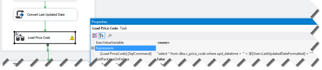
A Major League Baseball team engaged us to implement the foundation of their data analytics platform. They partner with TicketMaster for ticketing and sales. Interestingly, besides the TicketMaster cloud hosting that everyone is familiar with, Ticketmaster also offers a client application called Archtics to allow customers to sell tickets on premise. The client application uses a Sybase database (as you probably know, Sybase was acquired by SAP) that syncs with the host. Fortunately, Sybase and SQL Server has a lot in common but in the process we had to figure out a way to pull data from the Sybase database. To do so, you need to follow these steps:
Install the SQL Anywhere Database Client Download. During development, you will need the 32-bit driver because BIDS/SSDT is a 32-bit app. When running via SQL Server Agent, you’ll need the 64-bit driver.
Create an ODBC data source. Again you need to create two ODBC data sources using the 64-bit ODBC Administrator and then 32-bit ODBC Administrator.
Use the ODBC Source in SSIS to extract data from Sybase. Unfortunately, the ODBC Source doesn’t support parameterized statements, such as to extract data incrementally. As a workaround, you can use an expression-based SQL command text. You can do this by clicking on the Data Flow task in the package control flow and setting up an expression for the SQLCommand property.
Everyone wants to press a button and have the entire BI system generated and ready to go. But things are not that simple. You know it and I know it. Nevertheless, BI automation tools are emerging with growing promises that propelled them to the Top 10 BI Trends according to the Information Management magazine. As a side note, it was interesting that the same article put Big Data in the No 1 spot despite that Gartner deemphasized the Big Data hype (based on my experience and polling attendees to our BI group meetings, many don’t even know what Big Data is). While I don’t dismiss the BI auto-generators can bring some value, such as impact analysis and native support of popular systems, such as ERP systems, there are also well known cautions, include vendor lock-in, a new toolset to learn, suboptimal performance, supporting the lowest feature denominator of targeted database, etc. However, you don’t have to purchase a tool to save redundant implementation effort. Instead consider the following techniques:
Use the ELT (extraction, load, and transform) pattern instead or ETL (extract, transform, and load). While different solutions require different patterns, the ETL pattern is especially useful for data warehouse implementation because of the following advantages:
Performance – Set-based processing for complicated lookups should be more efficient than row-by-row processing. In SQL Server, the cornerstone of the ETL pattern is the T-SQL MERGE statement which resolves inserts, updates, and deletes very efficiently.
Features – Why ignore over two decades of SQL Server evolution? Many things are much easier in T-SQL and some don’t have SSIS counterparts.
Maintenance – It’s much easier to fix a bug in a stored procedure and give the DBA the script than asking to redeploy a package (or even worse a project now that we’ve embraced the project model in SSIS 2012).
Upgrading – As we’ve seen, SQL Server new releases bring new definitions that in many cases require significant testing effort. Not so with stored procedures.
Scalability – if you need to load fact tables, you’d probably need to do partitions switching. This is yet another reason to stage data first before you apply transformations.
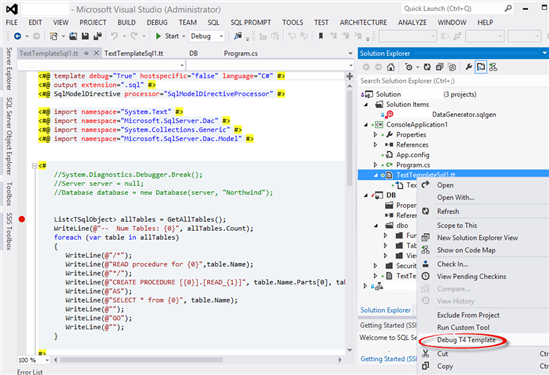
Automate the generation of stored procedure. The ELT pattern relies heavily on stored procedures. If you have to populate a lot of tables, consider investing some upfront development effort to auto-generate stored procedures, such as by using the Visual Studio Text Templates (also known as T4) templates. Note that to be able to debug them in Visual Studio 2012, you would need to add the template to a .NET project, such as a console application.
3. Automate the generation of SSIS packages. If you embrace the ELT pattern, your SSIS packages will be simple. That’s because most of the ELT code will be externalized to stored procedures and you would only use SSIS to orchestrate the package execution. Yet, if you have to create a lot of SSIS packages, such as to load an ODS database, consider automating the processing by using the Business Intelligence Markup Language (BIML) Script. BIML is gaining momentum. The popular BIDS Helper tool supports BIML. And, if you want to take BIMS to the next level, my friends from Varigence has a product offering that should help.
https://prologika.com/wp-content/uploads/2016/01/logo.png00Prologika - Teo Lachevhttps://prologika.com/wp-content/uploads/2016/01/logo.pngPrologika - Teo Lachev2014-05-11 19:42:002016-02-15 07:08:143 Techniques to Save BI Implementation Effort
At the Atlanta BI meeting last night, there was a question from the audience about differences between Inmon and Kimball and which methodology should be followed when implementing a data warehouse. I’ll recapture my thoughts and the feedback I shared.
As BI practitioners, most of us use methodologies and it’s easy to fall in love with a specific methodology. But sometimes methodologies conflict each other. So, don’t feel very strongly about methodologies. Instead, study them and try to synthetize their best. The best methodology is the one that delivers a business solution in the most practical and simple way. Back to Inmon vs Kimball, I have deep respect for both of them. They both contributed a lot to data warehousing that forms the backbone of modern BI. Both of these two methodologies aim to consolidate data and promote a single version of the truth. Both of them are “pure” database-focused and vendor-neutral methodologies for designing data structures. But they also differ in significant ways. This table summarizes the high level differences between the two methodologies.
Inmon
Kimball
APPROACH
Top-down Data warehouse first, data marts later
Bottom-up Data marts first, data warehouse later
SCHEMA
Normalized (3NF) schema
Denormalized (star) schema
HISTORY
All history needs to be captured
Depends on business requirements Type 1 vs Type 2 dimensions
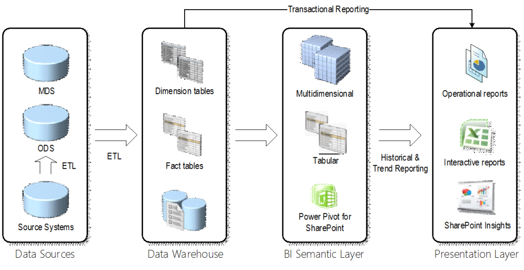
So, which one to follow? My answer is that there is a place for both. Consider the following BI architectural view.
Data comes from veriety of data sources. Some data, such as Products, Customers, Organizations, represents master data that should be ideally maintained in a separate repository, e.g. in Master Data Services. However, most of the source data is not master data and must be staged before it’s imported in the data warehouse. Instead of a transient staging database whose data is truncated with each ETL run, consider an ODS-style staging database that maintains historical changes.
Start_Date
End_Date
Store
Product
Deleted_Flag
1/1/2010
5/1/2010
Atlanta
Mountain Bike 1
5/2/2010
3/8/2012
Atlanta
Mountain Bike 2
3/9/2012
12/31/9999
Norcross
Mountain Bike 2
The Start_Date and End_Date columns are used to record the lifespan of each record and create row new versions each time the source row is changed. The example shows three changes that a given product has undergone. This design offers two main benefits:
1. It maintains a history of all changes that were made to all columns to all tables. Typically, OLTP systems don’t keep track of changes so the staging database can be used to record changes.
2. It maintains a full backup of the data. If a data warehouse needs to be reloaded, its history can be recreated from the staging database.
This ODS design is effectively your Inmon methodology in practice. For the data warehouse, I’d go with Kimball dimensional modelling. Dimensional modelling is a practical design technique whose goal is to produce a simple schema that is optimized for reporting. As far as data marts, I’m not so excited about moving data in or out of the data warehouse. In most cases, the most practical approach would be to implement a single data warehouse database and extend it as more subject areas come onboard. However, large organizations might benefit from data marts. For example, a large organization might have an enterprise data warehouse but for whatever reasons (usually IT not having enough resources), it might be difficult or not practical to extend it with a new subject areas. Then, this department might spin off its own data mart, such as on a separate database server (even from a different vendor, e.g. DW on Oracle and DM on SQL Server).
Ideally, the data mart should be able to reuse some of conformant dimensions from the data warehouse instead of implementing them anew. In reality, though, the enterprise bus could remain a wishful thinking. Having been left on his own devices, that department would probably need to implement the dimensions from the data they work with. For example, if this is an HR data mart, they would probably source an Organization dimension from PeopleSoft which is where their core data might come from.
With the risk of repeating myself, I want to reemphasize the role of the semantic layer which plays a critical role in every BI architecture. If you are successful implementing an enterprise bus consisting of a data warehouse and data marts (hub and spokes architecture), the semantic layer can provide a unified view the combines these data structures. For more information about the semantic layer benefits, refer to my newsletter “Why Semantic Layer“.
Using “smart” date surrogate integer keys in the format YYYYMMDD is a dimensional modeling best practice and venerable design technique. To make them smarter though, consider using the Date data type which was introduced in SQL Server 2008. The Date data type stores the date without the time component which is exactly what you need anyway. Using the Date data type instead of integers have the following benefits:
The Date data type allows you to perform date arithmetic easier as the date semantics is preserved, so you can use date functions, such as YEAR and MONTH when querying the table or partitioning a cube.
Self-service BI users can conveniently filter dates on import. For example, PowerPivot enables relative date filtering, such as Last Month, when the user filters a date column.
The Date data type has a storage of three bytes as opposed to four bytes for integers.
The only small downside of using the Date data type is that you will end up with funny looking unique names for the Date members in your Date dimension in an SSAS cube. The unique name will include the time portion, such as [Date].[Date].&[2013-07-01T00:00:00]. If you construct date members dynamically, e.g. to default to the current date, you have to append the time portion or use the Format function, such as Format(Now(),”yyyy-MM-ddT00:00:00″).
Scenario: Run ETL to perform a full data warehouse load. One of the steps requires joining four biggish tables in a stating database with 1:M logical relationships. The tables have the following counts:
VOUCHER: 1,802,743
VOUCHER_LINE: 2,183,469
DISTRIB_LINE: 2,658,726
VCHR_ACCTG_LINE: 10,242,414
Observations: On the development server, the SELECT query runs for hours. However, on the UAT server it finished within a few minutes. Both servers have the same data and hardware configuration, running SQL Server 2012 SP1.
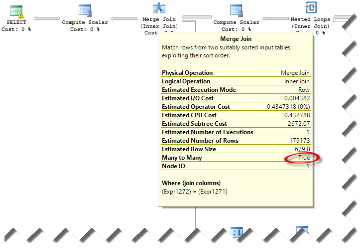
Solution: Isolating the issue and coming up with a solution wasn’t easy. Once we ruled out resource bottlenecks (both servers have similar configuration and similar I/O throughput), we took a look at the estimated query plan (we couldn’t compare with the actual execution plan because we couldn’t wait for the query to finish on the slow server).
We’ve notice that the query plans were very different between the two servers. Specifically, the estimated query plan on the fast server included parallelism and hash match join predicates. However, the slow server had merge M:M join predicates. This requires a tempdb work table for inner side rewinds which surely can cause performance degradation.
Interestingly, the cardinality of the tables and estimated number of rows didn’t change much between the two plans. Yet, the query optimizer decided to choose very different plans. At this point, we figured that this could be an issue with statistics although both servers were configured to auto update statistics (to auto-update statistics SQL Server requires modifications to at least 20% of the rows in that table). The statistics on the slow server probably just happened to have a sample distribution that led to a particular path through the optimizer that ended up choosing a serial plan instead of a parallel plan. Initially, we tried sp_updatestats but we didn’t get an improvement. Then, we did Update Statistics <table name> With Fullscan on the four tables. This resolved the issue and the query on the slow server executed in par with the query on the fast server.
Note: Updating statistics with full scan is an expensive operation that probably shouldn’t be in your database maintenance plan. Instead, consider:
1. Stick with default sampled statistics
2. Try hints for specific queries that exhibit slow performance, such as OPTION (HASH JOIN, LOOP JOIN) to preclude the expensive merge joins.
Special thanks to fellow SQL Server MVPs, Magi Naumova, Paul White, Hugo Kornelis, and Erland Sommarskog for shedding light in dark places!