Reporting on Concatenated Field in DAX
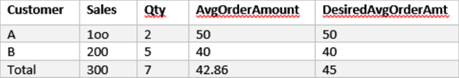
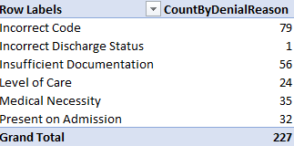
Scenario: You have a concatenated field stored in a table. For example, a medical claim might have several denial reasons. Instead of representing this as a Many-to-Many relationship, you’ve decided to store this a comma-delimited field, such as to allow the user to see all codes on one row. However, users are asking to produce counts grouped by each reason code, such as this one:
Solution: Follow these steps to implement a DAX measure that dynamically parses the string.
- Implement a DenialReason table with a single column DenialReason that stores the distinct reason codes. Add the table to your Power BI Desktop/Tabular model. Leaving it hanging without a relationship.
-
Add a CountByDenialReason DAX measure that parses the string:
CountByDenialReason :=
CALCULATE (
SUMX (
Claim,
IF (
NOT ISEMPTY (
FILTER (
VALUES ( DenialReason[DenialReason] ),
PATHCONTAINS (
SUBSTITUTE ( Claim[DenialReason], “,”, “|” ),
DenialReason[DenialReason]
)
)
),
1
)
)
)
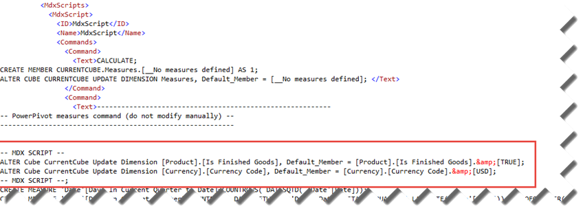
The NOT ISMPTY clause checks if the row contains any reasons. The PATHCONTAINS checks if the row has the denial reason whose context is passed from the report. In my case, the DenialReason field has a comma-delimited string if multiple reasons are stored on the row. Because PATHCONTAINS requires a pipe “|” delimiter, I use the SUBSTITUTE function to replace commas with pipes. If match is found for that reason, the IF operator returns one, which is summed in SUMX to return the actual count.
If you have a large table, you might get a better performance if you do the replacement in a wrapper SQL view or in Query Editor and avoid SUBSTITUTE altogether.