A scheduled SSIS job that executes a massive DAX query to an on-prem Tabular server (Power BI can also generate this error) one day decided to throw an error “Source: “Microsoft OLE DB Provider for Analysis Services.” Hresult: 0x80004005 Description: “MdxScript(Model) (2020, 98) Calculation error in measure ‘Account Snapshot'[Average utilisation % of all CR active current accounts last 3 months]: The result of a conversion or arithmetic operation is either too large or too small.” At least we know the offending measure, but which row is causing the error? The query requests some 300+ measures for 120 million customers, so I thought someone might find the troubleshooting technique useful. Let’s ignore what the measure does for now except mentioning that it performs a division of two other measures.
We can use the DAX ISERROR function to check if a measure throws an error. So, the first step is to wrap the measure with ISERROR and execute the query for all customers.
EVALUATE
FILTER (
 CALCULATETABLE (
 ADDCOLUMNS (
VALUES ( 'Customer'[Customer Registry ID] ),
"x", ISERROR ( [Average utilisation % of all CR active current accounts last 3 months] )
 ),
 FILTER ( VALUES ( 'Date'[Date] ), 'Date'[Date] = DATEVALUE ( "2022-10-14" ) )
 ),
 [x]
)
The query uses the ADDCOLUMNS function to add the measure so that it’s evaluated for each customer as of the date when the job ran. Make sure to add dependent measures that references the measure in the error description. ISERROR will return TRUE if the measure throws an error. The final step is to wrap CALCULATEDTABLE with FILTER that returns only the offending customer(s) where the measure is TRUE.
Using this technique, I’ve managed to narrow the error to data quality issues concerning large negative credit limits for some customers. BTW, the Tabular engine raises this error when converting a double precision floating point number to an integer, but the former is out of range of valid integer numbers.
A while back a client wanted to avoid importing a large snapshot fact table with loan balances because its memory footprint would require them to upgrade to a higher Power BI premium plan. This of course required leaving the table in DirectQuery mode at the expense of query performance. Luckily, most users would be interested in the latest six months of data. To speed up performance, we opted for aggregations. However, to complicate things further, they had M2M relationships between dimensions and the fact table which Power BI aggregations don’t support. So, we had to roll out our own “aggregation hits” by redirecting DAX measures either to the aggregated table if the as-of date was in the last six months or to the DirectQuery table otherwise.
Seasoned BI pros might recall that Multidimensional supports measure groups with a mixed storage by creating MOLAP and ROLAP partitions within the same table. The recently announced Power BI hybrid tables carry this concept to Tabular models hosted in Power BI Premium or PPU. This enables two new scenarios:
Implement real-time “hot” partitions – For best report performance, you can continue importing and refreshing the data periodically, but you can also implement a “hot” partition configured for DirectQuery to show the latest changes. This is the scenario supported by the incremental refresh policy discussed in the announcement.
Leave infrequently accessed data in DirectQuery – This is the scenario that I believe would inspire more interest to address the above requirement.
Implementing real-time partitions
The easiest way to implement a real-time partition is by defining an incremental refresh policy. All you must do is check the “Get the latest data in real time with DirectQuery” checkbox. This will add a DirectQuery partition to the end of the partition design created by Power BI. When the scheduled refresh runs, Power BI will refresh the historical partitions as it would normally do. However, all queries that request data after the scheduled refresh date (at the day boundary) will be sent to the data source. Consequently, your model will have new data that is inserted into the table. I suggest you also configure the report pages that show the real-time data for automatic page refresh (in Power BI Desktop, select the page and turn on the “Page refresh” slider) so that the visuals poll for data changes at a predefined cadence.
Leave infrequently accessed data in DirectQuery
Think of this scenario as the opposite of the real-time partitions because the frequently requested data is imported while the historical data is DirectQuery. Because Power BI Desktop doesn’t support custom partitions, you must use another tool, such as Tabular Editor or SSDT, to configure the partitions by connecting it to the published dataset via the XMLA endpoint (or working with a local *.bim file). If you prefer Power BI Desktop, another option could be to create the partitions in a published test or production model, use Power BI Desktop for development, and configure deployment pipelines to propagate the changes and preserve the partition design in the non-development environments. You’d probably need only two partitions:
Historical partition – Specify a SQL statement that queries the historical data with a WHERE clause that qualifies rows using a relative date, such as six months before the system date. Change the partition mode to DirectQuery.
Current partition – Specify a SQL statement that defines the slice for the frequently used data. Change the partition mode to Import.
Here are the high-level steps to implement the custom partition design with Tabular Editor assuming you would create the partitions in a published dataset. Note that the first step use Power BI Desktop. You can use Tabular Editor for all steps but it’s a more advanced tool so you might want to use something you’re more familiar with.
Start by opening your dataset in Power BI Desktop. For best performance, drop all imported dimension tables that relate to the large fact table, reimport them in DirectQuery, and then change their storage mode to Dual. That’s because currently Power BI Desktop doesn’t let you switch from Import to DirectQuery and there is no workaround.
Open the Power Query Editor. By default, every table will have one partition and if you used Power BI Desktop, the partition will be an M partition (meaning it will have a Power Query). Change the Source step of the first partition to use a custom query (click the gear icon next to the Source step and then enter your custom SQL statement as per you requirements. For example, if you want the default partition to import the last six months and you target SQL Server, the Source step might look like this:
let
Source = Sql.Database("XPS", "AdventureWorksDW2012", [Query="select * from FactResellerSales where OrderDate >= DATEADD(month, -6, GETDATE())"])
in Source
Publish the dataset to Power BI Service. Close Power BI Desktop and promise yourself never to use it again for that dataset (if you can’t live without it, see the aforementioned note about deployment pipelines). That’s because if you republish the model, PBI Desktop will nuke the custom partitions in the deployed dataset (nice work here Microsoft). Remember that the only partition design supported and preserved by Power BI Desktop is the incremental refresh policy but you can’t use incremental refresh for this scenario.
Connect the Tabular Editor to the published dataset XMLA endpoint (File, Open, From DB). As a prerequisite, make sure to enable the XMLA Endpont for Read/Write in the capacity settings.
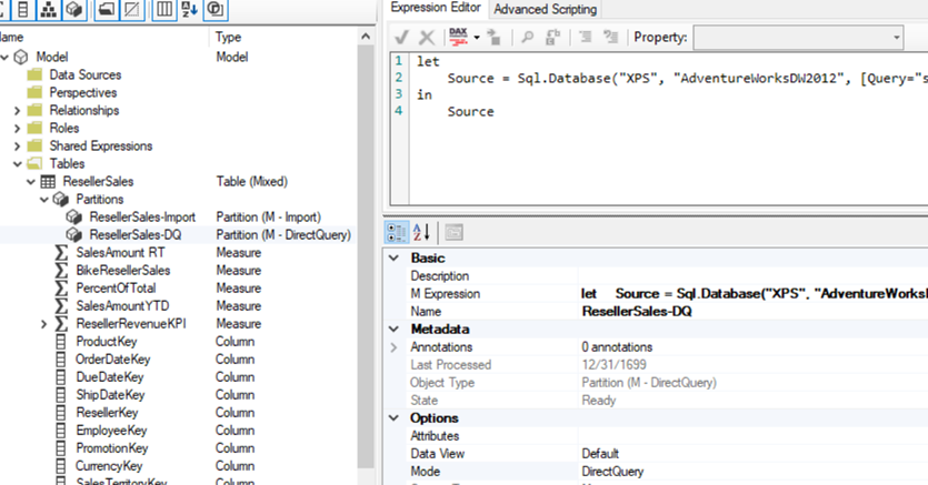
Rename the first partition, e.g. ResellerSales-Import.
Duplicate the partition and rename the second one ResellerSales-DQ. Change its Mode property to DirectQuery. Change its source query to slice the historical data.
let
Source = Sql.Database("XPS", "AdventureWorksDW2012", [Query="select * from FactResellerSales where OrderDate < DATEADD(month, -6, GETDATE())"])
in Source
Save (or deploy) the changes to Power BI Service and refresh the dataset.
(Optional) Open SQL Server Profiler connected to the published dataset. User Power BI Desktop or Analyze in Excel to create a report that queries the fact table by date. Notice that when the date filter falls within the last six months, there are no events in the profiler because the query is answered by the Tabular cache. However, when the date filter is outside that period, the profiler shows a SQL SELECT statement because that data is left in the data source to reduce the model’s memory footprint at the expense of performance.
This is what your partition design should look like:
Hybrid tables go even further than composite models by allowing you to mix storage modes within a table and having partitions in Import or DirectQuery storage modes. They enable two scenarios: real-time “hot” partitions and leaving infrequently accessed data in DirectQuery data. What I would like to see Microsoft improve in future is a) let us switch from Import to DirectQuery although this might break calculated columns and Power Query transforms, b) extend Power BI Desktop to support custom partitions so that we can connect Tabular Editor as an external tool and change the partition design and save it in the pbix file, and c) extend Power BI Desktop to preserve the partition design on deploy.
I hope you’re enjoying the holidays. In this newsletter, I’ll discuss a very important enhancement to Power BI that lets business users extend semantic models. But before I get to it, a quick announcement. I’m putting the finishing touches of the sixth edition of my “Applied Microsoft Power BI”! It should be available on Amazon in the first days of 2021. I’ve been updating this book thoroughly every year since 2015 to keep it up to the date with this fast-changing technology.
I’ve written extensively on the important role that EDW and organizational semantic models have for delivering the “Discipline at the core and flexibility at the edge” tenant for effective data analytics. Analysis Services Tabular is available in three SKUs: Power BI, Azure Analysis Services, and SSAS, and it’s the workhorse of Power BI Service. When you publish a Power BI desktop file, it becomes a database hosted in some Analysis Services Tabular server managed by Microsoft.
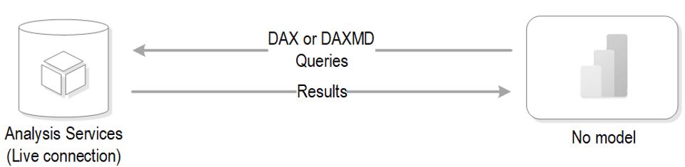
How live connections work
As the diagram below shows, Power BI uses a special live connectivity option when you connect live to Analysis Services in all its flavors (Multidimensional, Tabular, and Power BI published datasets) and SAP (SAP Hana and SAP Data Warehouse). In this case, the xVelocity engine isn’t used at all and the model is absent. Instead, Power BI connects directly to the data source and sends native queries. For example, Power BI generates DAX queries when connected to Analysis Services .
There is no Power Query in between Power BI Desktop and the data source, and data transformations and relationships are not available. In other words, Power BI becomes a presentation layer that is connected directly to the source, and the Fields pane shows the metadata from the model. This is conceptually very similar to connecting Excel to Analysis Services.
Unfortunately, once you connected Power BI Desktop to a multidimensional data source, that remote model was the only data source available for you.
Understanding the change
Power BI Desktop (December 2020 release) removes this long-standing limitation for live connections to Tabular. In the special case of connecting to a dataset published to Power BI Service and Azure Analysis Services (on-prem SSAS is not supported), you can switch from live connectivity to DirectQuery and add external data to build a composite model. This feature is very important because it allows business users to extend semantic models that could be sanctioned by someone else in the organization!
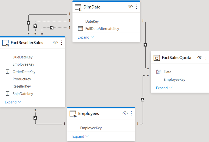
If the first connection you make is to the remote model then the connection will use Live Connect. The Power BI Desktop file will not store any metadata or data, expect for the connection string. The moment you use “Get Data” to connect to another source and accept the prompt, Power BI Desktop replaces permanently the live connection with a local DirectQuery layer and imports the metadata of the remote model. Even if you remove all external tables, you won’t be able to “undo” the change and switch back the file to Live Connect. In the diagram below, FactResellerSales, DimDate, and Employees tables are hosted in the remote model while FactSalesQuota is an external table that is imported (could be in DirectQuery mode).
What happens behind the scenes
In a nutshell, DirectQuery to Analysis Services Tabular is like other DirectQuery sources where DAX queries generated by Power BI are translated to native queries. However, in this case Power BI either sends the DAX queries directly to the remote model when possible or breaks them down into lower-level DAX queries. In the latter case, the DAX queries are executed on the remote model and then the results are combined in Power BI to return the result for the original DAX query. So, depending on the size of the tables involved in the join, this intermediate layer may negatively impact performance of visuals that mix fields from different data sources.
Applying your knowledge about composite models, you might attempt to configure the dimensions in dual storage, but you’ll find that this is not supported. Behind the scenes, Power BI handles the join automatically, so you do not need to set the storage mode to Dual. It’s interpreted as Dual internally. You can make metadata changes on top of the remote model. For example, you can format fields, create custom groups, implement your own measures, and even calculated columns (calculated columns are now evaluated at runtime and not materialized). The changes you make never affect the remote model. They are saved locally in the DirectQuery model.
Currently, row-level security (RLS) doesn’t propagate from the remote model to the other tables. For example, the remote model might allow salespersons to see only their sales data by applying RLS to the Employees table. However, the user will be allowed to see all the data in the FactSalesQuota table because it’s external to the remote model and RLS doesn’t affect it.
Teo Lachev Prologika, LLC | Making Sense of Data Microsoft Partner | Gold Data Analytics
I am delivering a data governance assessment for an enterprise client. As a part of the effort to migrate reporting from MicroStrategy to Power BI, the client wants to improve data analytics. The gap analysis interviews with the business leaders revealed common pitfalls: no single version of truth, data is hard to come by, business users don’t know what data sources exist, business users spend more time in data wrangling than analytics, data quality is bad, IT is overwhelmed with report requests, report proliferation and duplication, and so on…
Sounds familiar? As I mentioned many times in my blog, an enterprise data warehouse (EDW) plays a critical role in overcoming the above challenges, but it’s not enough. A semantic model is needed and I extolled its virtues in my “Why Semantic Layer?” newsletter. In the Microsoft BI world, Analysis Services Tabular is commonly used to implement such models that are typically layered on top of EDW . In general, there are two ways to approach the model implementation:
(Self-service BI path) Business users create self-service semantic models using Power BI Desktop. Behind the scenes, Power BI creates databases hosted in the Analysis Services Tabular server from the *.pbix files.
(Organizational BI path) BI developers implement organizational semantic models.
Since both implementation paths lead to the same technology, it boils down to ownership, vision, and purpose.
Because IT is overwhelmed, the temptation is to transfer the semantic model development to business users. The issue with this approach is business users seldom have the skills, time, and vision to do so. And the end, mini “semantic models” (“spreadmarts”) are produced and the same problems are perpetuated.
In most cases, my recommendation is for IT to own the semantic model because they own the data warehouse and the “Discipline at the Core” vision. And yes, unless operational and security requirements dictate otherwise, it should strive for a single centralized semantic model that spans all subject areas. If the technology you use for semantic modeling can’t deliver acceptable performance with large models, then it’s time to change it.
Of course, not all data exists or will exist in EDW. This is where self-service “Flexibility at the Edge” comes in. I have high expectations for the forthcoming “Composite models over Power BI datasets and Azure Analysis Services” mega feature (public preview expected in November 2020). This will enable the following scenario that Power BI cannot deliver today:
Business user starts by connecting live to corporate data in the organizational semantic model. Every new report requirement should start with evaluating if all or some of the data is in the semantic model, and if so, instructing the user to connect to the semantic model to avoid data modeling and data duplication.
Business user wants to mash up this data with some data that is not in EDW by retaining the live connection to the organizational semantic model and importing (or connective live with DirectQuery) to other datasets.
In my previous post about responsive reports, I said that changes to the report design can dramatically reduce the report load time. But you will undoubtedly reach a point where you cannot optimize the report any further. After all, having a page with a single visual might be fast, but I doubt it would deliver much business value. What else can be done to speed up the reports and ideally achieve a page load time of a few seconds? Our next stop for that project is to revisit the solution architecture. The client initially opted for a hybrid architecture where the reports use live connection to on-prem SSAS Tabular models. However, a significant time was spent in Power BI showing “loading data” before rendering the report. What took so long?
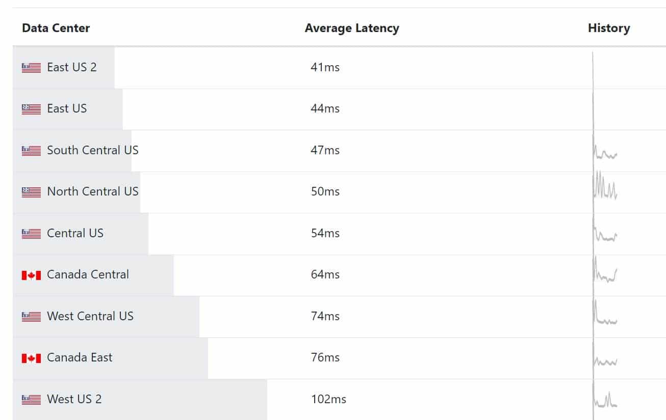
In this case, Power BI was hosted in the Azure West region, the Tabular server in the company data center in Atlanta, and most users were in the East region. This resulted in round trips crossing the country for each visual.
A user in the East region requests a report which is hosted in the West region.
Each visual generates a query which is sent to Tabular in the company data center.
SSAS returns data back to the West region.
Report payload is sent to the user in the East region.
Ideally, users, reports, and data should be in the same region. However, a long-standing limitation of Power BI is that once the first user signs up for Power BI, Power BI determines the data region based the user location and you can’t move it unless you open a support ticket with Microsoft. Power BI Premium will let you create premium capacities in a different region, but by default these capacities will be created in the original Power BI region and you can’t change the region once the capacity is created either. The chart below shows the round-trip latency doubles if the user is in the East region, but Power BI is in the West.
We decided to move the semantic model to Power BI so that Power BI owns the data. Besides potentially improving the report load time, this architecture has also other important advantages (to learn more, read my “Power BI Large Datasets: The Good, the Bad, and the Ugly” post). If you’re not on Power BI Premium, that “movement” might not easy if you have opted to use Visual Studio or Tabular Editor for development. That’s because Power BI Pro doesn’t expose the XMLA endpoint, so your only option is to migrate the model to Power BI Desktop. But migrating an SSAS Tabular project to Power BI Desktop is not officially supported and there is no automatic migration path.
Thanks to the enhanced dataset metadata (a better name would have been “metadata done right this time”), you could opt for cracking the Power BI Desktop file and replacing the model schema (my “Power BI Source Control” blog has the steps to get to the schema). You might get lucky especially if your Tabular project uses structured data source (the only data source type supported by Power BI Desktop). However, if it uses legacy data sources, you must change every table to use a structured data source and making changes to the JSON schema by hand and Power BI Desktop refusing the load the model with every typo is no fun.
On the other hand, Power BI Premium lets you deploy the SSAS model to the workspace XMLA endpoint. The prerequisites are:
Upgrade the Tabular model in Visual Studio to 1500 compatibility mode. This adds special annotations to the data source. If you don’t upgrade to 1500, you’ll find that you won’t be able to schedule the dataset for refresh as Power BI Service won’t show any connections.
Enable the XMLA endpoint for read-write in the capacity settings.
Enable the “Export data” tenant setting in Power BI (to learn more about this setting, read my “A False Sense of Security” blog).
Like the “Export data” battle wasn’t enough, we found that we have to beg the Security group to enable also the “Analyze in Excel with on-premise datasets” tenant setting. I have no idea what this setting has to do with the XMLA endpoint. Luckily, Fidler showed us the exact error message that this setting must be enabled.
Moving the semantic model paid big dividends. We could only see “loading data” for a moment. We also found that the network speed of the user connection and the browser play a significant role. For best performance, users should use Chrome or new Edge and have a broadband connection. We were able to reduce further the load time of the first page by enabling the published dataset for query caching which is only available in Power BI Premium.
https://prologika.com/wp-content/uploads/2016/01/logo.png00Prologika - Teo Lachevhttps://prologika.com/wp-content/uploads/2016/01/logo.pngPrologika - Teo Lachev2020-07-06 14:57:282020-07-06 14:57:28Designing Responsive Power BI Reports (Part 2)
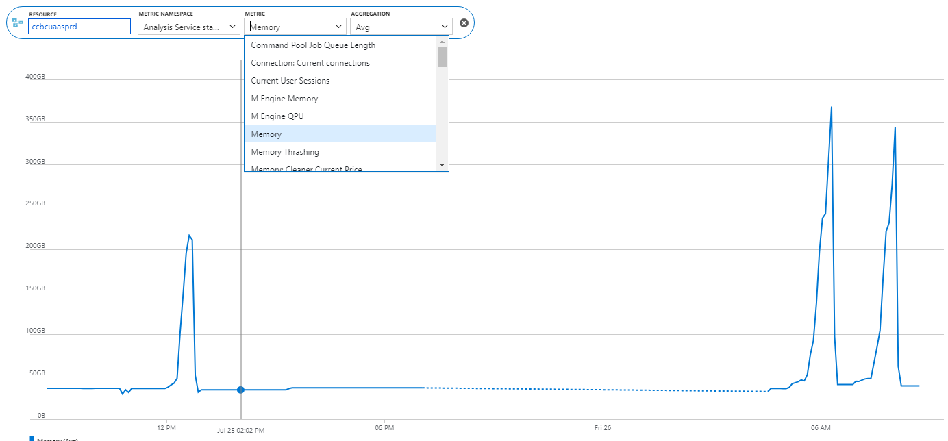
Scenario: A client reports a memory spike during processing. They have a Tabular semantic model deployed to Azure Analysis Services. They fully process the model daily. The model normally takes less than 50 GB RAM but during processing, it spikes five times and Azure Analysis Services terminates the processing task complaining that it “reached the maximum allowable memory in our pricing tier”. Normally, fully processing the model should take about twice the memory but five times?
Solution: Upon expecting the model design, I discovered that the client has decided to add (many) calculated columns to the two fact tables in the model. Most of these columns are used to calculated variances to prior year. The formulas contain DATESYTD and other DAX date-related functions. After data is read, Tabular processes calculated columns, relationships and hierarchies. In this case, the spike was due to calculations involving large time ranges and ineffective DAX expressions. Converting these columns to measures resolved the issue.
As a best practice, abstain from using calculated columns (especially in fact tables). Make sure you understand the difference between measures and calculated columns (I cover this extensively in my latest book “Applied DAX with Power BI“). If you do need expression-based columns, such to materialize expensive calculations, consider defining them upstream, such as in SQL views or Power Query.
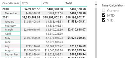
Just when I started thinking that there won’t be any new BI features in SQL Server 2019, Christian Wade announced DAX calculation groups in CTP 2.3. His excellent post helped me try them out with Tabular Editor and Power BI Desktop and whip out this cool report.
As Chris Webb pointed out, DAX calculation groups let us implement time calculations as in Multidimensional with a “shell” time dimension. They probably won’t help you reducing the number of measures because you’d still need to flatten the “shell” dimension for maximum flexibility and avoid forcing the user to use the Time Calculations slicer to select the time calculations they want on the report. So, you would still have to project Sales Amount YTD as a separate measure:
What calculation groups help with is avoiding copying and pasting the time intelligence formulas all over the place. A future CTP will also help centralize measure formatting where you’ll have the option to inherit the current measure format string (by leaving it blank), or override it.
To me, DAX calculation groups is a nice to have feature, which I could have happily traded for more significant ones. Speaking of which, I hope Microsoft adds more important enhancements to Tabular 2019.
Here is my top 10:
Anything that can help the poor developer debug and understand in what context a DAX expression is evaluated as DAX tends to have more exceptions than rules.
DAX script – to show and organize all measures in one place. I miss also the MD scope assignments.
What tool do you use for Analysis Services Tabular development? SSDT right, what else? Here is a little secret. I almost don’t use SSDT anymore, except for limited tasks, such as importing new tables and visualizing relationships. I switched to a great community tool – Tabular Editor and you should too if you’re frustrated with the SSDT Tabular Designer. Back in 2012 Microsoft ported the Power Pivot designer to SSDT to let BI practitioners implement Tabular models. This is why you still get weird errors that Excel has encountered some error. Microsoft haven’t made any “professional” optimizations despite all the attention that Tabular gets. As a result, developers face:
Performance issues – As your model grows in complexity, it gets progressively slower for even simple changes, such as renaming columns. The problem of course is that any change results in a commit operation to the workspace database. SSDT requires a workspace database for the Data View but it slows down all tasks even if it doesn’t have data. While the data view is useful for data analysts, I’d personally rather sacrifice it to gain development speed.
The horrible measure grid – Enough said. To Microsoft credit, the Tabular Explorer helps somewhat but it still doesn’t support the equivalent of the SSAS MD script editor.
No automation for repetitive tasks – It’s not unusual to create many measure variants, such as YTD, QTD. SSDT doesn’t help much automating them.
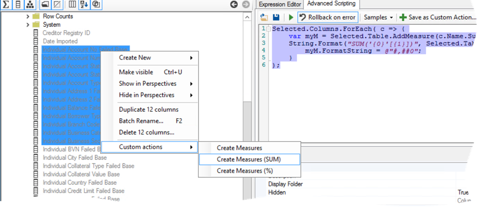
Tabular Editor to the rescue! It will probably take you some time to get used to it and as the author, Daniel Otykier, admits “…the tool is probably not well-suited for first time Tabular developers”. But once you get used to it you probably won’t go back to SSDT. No more workspace databases and lightning fast performance! And the cherry on top of the pie is that you can write scripts to automate repetitive tasks. Say for example, you have a bunch of base numeric columns you want to convert to explicit measures to make Excel happy (don’t get me started on the Excel support for Tabular). What is a developer to do? Write some code of course. With some C# knowledge, you whip out the following script:
Selected.Columns.ForEach( c => {
var myM = Selected.Table.AddMeasure(c.Name.Substring(0, c.Name.Length-5),
This script enumerates through the selected columns and create a measure for each column that sums the underlying column. For example, if the base column is Sales Amount Base in table Reseller Sales, the script will create a measure Sales Amount = SUM(‘Reseller Sales'[Sales Amount]). Then, you can save the script as a custom action (not be confused with AS actions). Then, select all the “base” columns, invoke the custom action and voila! – you get all the measures autogenerated! You can then select all these measures and change their properties, such as assign them all to a display folder. You also have much better control over deploying your changes to the server. Everything is simple with Tabular Editor.
Tabular Editor is a great community tool that can help you implement and maintain Tabular models much faster than SSDT. I highly recommend it if you’re frustrated with the SSDT developer experience. Kudos to Daniel Otykier and the other community members who contributed to this tool.
Problem: A long standing limitation in Analysis Services Tabular and Power BI is the lack of default members, such as to default a Date dimension to the last date with data. Users find this annoying, especially for time calculations which require a date context and won’t produce results until you add a date-related field to the report one way or other. To aggravate things even more, Tabular switched to a JSON schema in SQL Server 2016. The new schema is great for expressing the metadata in clear and more compact way. However, because it’s not extensiible, it precludes community tools, such as BIDS Helper (now called BI Developer Extensions) and DAX Editor, to extend Tabular features and fill in the gaps left by Microsoft.
Workaround: Currently, there is no way to default a field in Tabular and Power BI. For the most common requirement to default a date filter, consider adding a field to the Date table that flags the desired item. You can implement this in different ways. For example, in Excel you can create a named set, but this requires MDX knowledge that end users won’t have. And it won’t work in other report clients, such as Power BI Desktop. Here is an approach that is simple to implement and works everywhere.
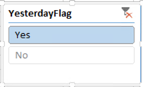
Flag the desired item using whatever way you’re comfortable with: SQL view, Power Query, or DAX. For example, if users prefer the date filter to default to yesterday and the Date table is based on a SQL view, add the following column to the view: CASE WHEN [Date] <= DATEADD(DAY,-1, CAST(GETDATE() AS DATE)) THEN ‘Yes’ ELSE ‘No’ END YesterdayFlag Notice that the flag qualifies all rows prior to and including yesterday. In your first attempt, you might try only an equal condition. This will work when the YesterdayFlag field is added as a filter to an Excel pivot table. However, if you attempt to configure it as an Excel slicer, it will result in the following error: Calculation error in measure ‘<your measure name>’: Function ‘SAMEPERIODLASTYEAR’ only works with contiguous date selections.
Reimport the Date table in Tabular or Power BI.
Set up a report filter. For example, in Excel define a slicer using the YesterdayFlag field and default it to Yes, if you want to filter all reports on the same sheet.
The net effect is that as time progresses, the YesterdayFlag field will filter the Date table and measures will show the yesterday’s data by default. Time calculations will also work as of yesterday. For example, YTD calculations will aggregate from the beginning of the year until yesterday. And end users don’t need to bother about resetting date filters if viewing data as yesterday is the prevailing preference.
https://prologika.com/wp-content/uploads/2016/01/logo.png00Prologika - Teo Lachevhttps://prologika.com/wp-content/uploads/2016/01/logo.pngPrologika - Teo Lachev2018-07-18 21:20:292018-07-20 14:01:57Implementing a Default Date Filter in Tabular and Power BI