A First Look at Power BI Aggregations

During the “Building a data model to support 1 trillion rows of data and more with Microsoft Power BI Premium” presentation at the Business Applications Summit, Microsoft discussed the technical details of how the forthcoming “Aggregations” feature can help you implement fast summarized queries on top of huge datasets. Following incremental refresh and composite models, aggregations are the next “pro” feature that debuts in Power BI and it aims to make it a more attractive option for deploying organizational semantic models. In this blog, I summarize my initial observations of this feature which should be available for preview in the September release of Power BI.

Aggregations are not a new concept to BI practitioners tackling large datasets. Ask a DBA what’s the next course of action after all tricks are exhausted to speed up massive queries and his answer would be summarized tables. That’s what aggregations are: predefined summaries of data, aimed to speed queries at the expense of more storage. BI pros would recall that Analysis Services Multidimensional (MD) has supported aggregations for a long time. Once you define an aggregation, MD maintains it automatically. When you process the partition, MD rebuilds the partition aggregations. An MD aggregation is tied to the source partition and it summarizes all measures in the partition. You might also recall that designing proper aggregations in MD isn’t easy and that the MD intra-dependencies could cause some grief, such as processing a dimension could invalidate the aggregations in the related partitions, requiring you to reprocess their indexes to restore aggregations. On the other hand, as it stands today, Analysis Services Tabular (Azure AS and SSAS Tabular) doesn’t support aggregations. Power BI takes the middle road. Like MD, Power BI would search for suitable aggregations to answer summarized queries, but it requires more work on your part to set them up.

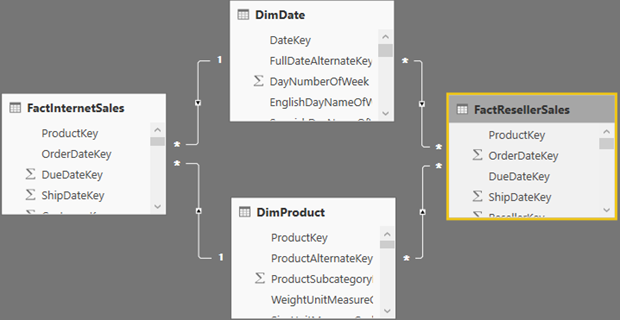
Consider the following model which has a FactInternetSales fact table and three dimensions: DimCustomer, DimProduct, and DimDate. Suppose that most queries would request data at the Product and Date levels (not Customer) but such queries don’t give you the desired performance. This could be perhaps because FactinternetSales is imported (cached) but it’s huge. Or, FactInternetSales could be configured for DirectQuery but the underlying data source is not efficient for massive queries. This is where aggregations might help (contrary reasons for using aggregations is to compensate for bad design or inefficient DAX).

081318_1754_AFirstLooka1.png

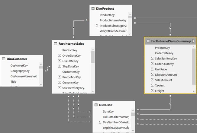
As a first step for setting up aggregations, you need to add a summarized table. Unlike MD, you are responsible for designing, populating and maintaining this table. Why not the MD way? The short answer is flexibility. It’s up to you how you want to design and populate the summarized table: ETL or DAX. It’s also up to you which measures you want to aggregate. And, the summarized table doesn’t have to be imported (it could be left in DirectQuery). You can also have multiple aggregations tables (more on this in a moment). In my case, I’ve decided to base the FactInternetSalesSummary table on a SQL view that aggregates the FactInternetSales data, but I could have chosen to use a DAX calculated table or load it during ETL. In my case, FactInternetSalesSummary aggregates sales at the Product and Date level, assuming I want to speed up queries at that grain. In real life, FactInternetSalesSummary would be hidden to end users so they are not confused which table to use.

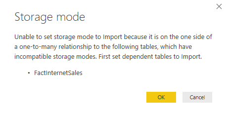
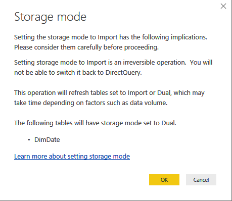
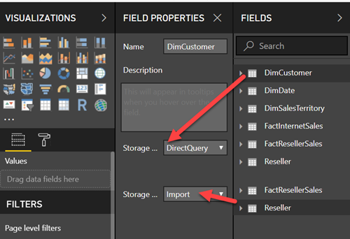
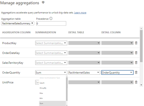
Note that a composite model has specific requirements for configuring dimension tables, which I discussed in my blog “Understanding Power BI Dual Storage“. For example, if FactInternetSalesSummary is imported but FactInternetSales is DirectQuery, DimProduct and DimDate must be configured in Dual storage mode. Once the aggregation table is defined, the next step is to define the actual aggregations. Note that this must be done for the aggregation table (not the detail table) so in my case this would be FactInternetSalesSummary. Configuring aggregations involves specifying the following configuration details in the “Manage aggregations” window:

  • Aggregation table – the aggregation table that you want to use for the aggregation design.
  • Precedence – in the case of multiple aggregation tables, you can define which aggregation table will take precedence (the server will probe the aggregation table that has a highest level first). Another feature that opens interesting scenarios.
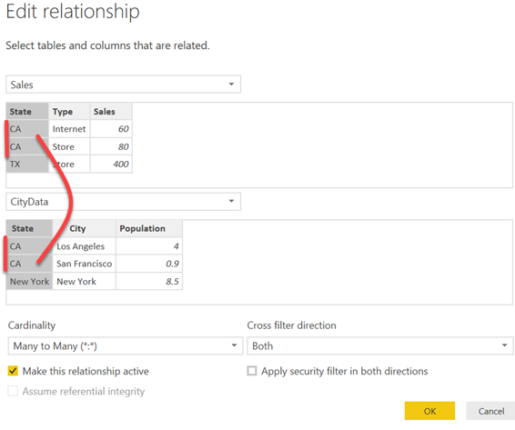
  • Summarization function – Supported are Count, GroupBy, Max, Min, Sum, Count. If the aggregation table has relationships to dimension tables, there is no need to specify GroupBy. However, if the aggregation table can’t be joined to the dimension tables in a Many:1 relationship, GroupBy is required. For example, you might have a huge DirectQuery table where all dimension attributes are denormalized and another summarized table. Because currently aggregations don’t support M:M relationships, you must use GroupBy. Another usage scenario for GroupBy is for speeding up DistinctCount measures. If the column that the distinct count is performed is defined as GroupBy, then the query should result in an aggregation hit. Finally, note that derivative DAX calculations that directly or indirectly reference the aggregate measure would also benefit from the aggregation.
  • Detail table – which table should answer the query for aggregation misses. Note that Power BI can redirect to a different detail table for each measure. Even more flexibility!
  • Detail column – what is the underlying detail column.

081318_1754_AFirstLooka2.png

The next step is to deploy the model and schedule the aggregation table for refresh if it imports data. Larger aggregate tables would probably require incremental refresh. Once the manual part is done, the server takes over. In the presence of one or more aggregation tables, the server would try to find a suitable table for aggregation hits. You can’t discover aggregation hits in the SQL Server Profiler by monitoring the existing MD “Getting Data from Aggregation” event. Instead, a new ” Query Processing\Aggregate Table Rewrite Query” event was introduced:

{

“table”: “FactInternetSales”,

“mapping”: {

“table”: “FactInternetSalesSummary”

},

“matchingResult”: “matchFound“,

“dataRequest”: [

}

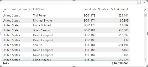
To get an aggregation hit at the joined dimensions granularity, the query must involve one or more of the actual dimensions. For example, this query would result in an aggregation hit because it involves the DimDate dimension which joins FactInternetSalesSummary.

EVALUATE
SUMMARIZECOLUMNS (
‘DimDate'[CalendarYear],
“Sales”, SUM ( FactInternetSales[SalesAmount] )
)

However, this query won’t result in an aggregation hit because it aggregates using a column from the InternetSales table, even though this column is used for the relationship to DimDate and the aggregation is at the OrderDateKey grain.

EVALUATE
SUMMARIZECOLUMNS (
FactInternetSales[OrderDateKey],
“Sales”, SUM ( FactInternetSales[SalesAmount] )
)

Aggregations are a new feature in Power BI to speed up summarized queries over large or slow datasets. Microsoft has designed aggregations with flexibility in mind allowing the modeler to support different scenarios.

Understanding Power BI Dual Storage

The July release of Power BI Desktop introduced composite models, which I wrote about in my blog “Power BI Composite Models: The Good, The Bad, The Ugly” Composite models make data acquisition much more flexible but also more complex. A Power BI table can now be configured in one of these storage modes:

  • Import – The table caches the data. All Power BI features work.
  • DirectQuery – The table has only the metadata while the data is left at the data source. When users interact with the report, Power BI generates DAX queries to the Analysis Services server hosting the model, which in turn generates native queries to the data source. DirectQuery supports limited Power Query transformations and DAX functions in calculated columns, as described in more details here. Besides Power Query and DAX limitations, DirectQuery and Live Connections have feature limitations, as I discussed in my blog “Power BI Feature Discrepancies for Data Acquisition“.
  • Live Connection – This is a special case when Power BI connects directly to multidimensional data sources, such as Analysis Services, published Power BI Datasets and SAP Hana. The fact that Power BI doesn’t support DirectQuery against these data sources is the reason why composite models are not supported as well.
  • Dual – This is a new storage mode that deserves more attention.

As the name implies, the dual storage mode is a hybrid between Import and DirectQuery. Like importing data, the dual storage mode caches the data in the table. However, it leaves it up to Power BI to determine the best way to query the table depending on the query context. Consider the following schema where all tables come from the same data source. Let’s assume the following configuration:

  • FactInternetSales is imported
  • FactResellerSales is DirectQuery
  • DimDate and DimProduct are Dual

080518_2257_Understandi1.png

Power BI will attempt the most efficient was to resolve the table joins. For example, if a query involves FactInternetSales and one or more of the dual dimensional tables, such as DimDate, the query would involve the DimDate cache. However, if the query involves FactResellerSales, Power BI will pass through the join. That’s because it would much more efficient to let the data source join the two tables in DirectQuery as opposed to bringing all the FactResellerSales table at the join granularity and then joining to the DimDate cache. In fact, Power BI will force you to change related dimension tables to Dual when it discovers hybrid joins among tables in the same data source. The following storage mode configurations are allowed between any two tables participating in M:1 join from a single data source:

Table on Many Side Is InTable on One Side Must Be In
DualDual
ImportImport or Dual
DirectQueryDirectQuery or Dual

Therefore, a conformed dimension table must be configured for a Dual mode to join a fact table in Import mode and a fact table in DirectQuery mode.

When Power BI Desktop detects an incompatible configuration, it may disallow the change. It may disallow the configuration because currently Power BI can’t switch from Import to any other storage mode.

Or, it may ask you to switch storage modes it if finds a way to perform the change on its own.

Dual mode is important for tables coming from a single data source. Heterogeneous joins spanning two data sources would always result in a M:M relationship where the Power BI Mashup Engine will resolve the join. Specifically, when the joined table cardinality exceeds an undisclosed by Microsoft threshold, Power BI would perform the join on its own. For example, if DimDate is imported from Data Source A but FactResellerSales is DirectQuery in Data Source B, Power BI would send a direct query to group FactResellerSales to B at the join cardinality (e.g. DateKey), get the data, and then join the tables internally.

On my question why Power BI doesn’t handle the dual storage mode on its own by selecting the most efficient join, Microsoft replied that there are two reasons to delegate this task to the modeler and to make the Dual storage configuration explicit:

  • Like Import, Dual requires refresh, whereas DirectQuery doesn’t.
  • Apart from being able to revert to DirectQuery mode, Dual is subject to the same restrictions as DirectQuery.

Therefore, the modeler needs to be aware that the “switch” may result in requiring a data refresh or may result in a data a loss.

The Power BI dual storage mode is important when creating 1:M joins between tables in different storage modes from the same data model and for the forthcoming “Aggregations” feature, which I’ll cover in another blog. Although you need to know how Dual works, you don’t need to remember rules as Power BI Desktop will detect incompatible configurations. Composite models, heterogeneous M:M relationships, dual storage mode, and aggregations are Power BI-only features. At this point, Microsoft hasn’t announced when they will be available in Azure Analysis Services or SSAS Tabular.

Great Atlanta MS BI and Power BI Group Meeting Last Night

A good turnout last night for our Atlanta MS BI and Power BI Group July meeting. Some 60+ attended the meeting at the MTC office at Avalon. Kudos to Scott Fairbanks for the great presentation and CCG for sponsoring the meeting. Thanks to Microsoft for hosting us. We’ll make the slides available shortly at http://atlantabi.pass.org/Resources.aspx.

Power BI News from the Microsoft Business Applications Summit

If you haven’t done so, watch the “Power BI and the Future for Modern and Enterprise BI” presentation from the Business Applications Summit (July 22-24) to find where Microsoft is bringing Power BI in the next few months.

Power BI Service Scale and Adoption

  • 19M data models hosted
  • 58M monthly publish to web views
  • 8M+ report and dashboard queries/hour
  • Power BI a top 10 fastest growing skill according to Upwork

Microsoft will extend Power BI by investing in three main areas:

  • Unified platform for both self-service and enterprise BI
  • Intuitive experience that drive a data culture
  • Pervasive Artificial Intelligence for BI

072818_1802_PowerBINews1.png

Here are most important forthcoming near-future features across these three areas:

Unified platform for both self-service and enterprise BI

  • Make Power BI Desktop a better tool for larger models — new diagram view with perspectives, multi-select fields to set common properties (it’s about time to have this feature), display folders as in SSAS
  • Composite models (delivered in July 2018 release) – I covered this killer feature in my blog “Power BI Composite Models: The Good, The Bad, The Ugly
  • Aggregations – Ability to define aggregations as we can do in SSAS MD. The demo showed an impressive response time for summarized views on top of a 1 trillion row dataset.
  • Multi-geo deployments

Intuitive experience that drive data culture

  • Certified datasets
  • Application lifecycle managements (DEV, QA, PROD environments)
  • Dataflows – dataflows refer to what was announced as “datapools” and Common Data Model for Analytics (review my comments here).
  • Modernized Visualizations pane (delivered in July 2018 release)
  • Report wallpaper (delivered in July 2018 release)
  • Out of box themes
  • Visual headers (delivered in July 2018 release)
  • Snap visual with other visuals
  • Expression-based formatting for every property in the Visualizations pane – This is huge and my users would rejoice to have more control over report properties!
  • Excel-like pivot tables
  • Export to PDF – most voted feature will finally be delivered

Pervasive Artificial Intelligence for BI

  • Quick Insights on right-click
  • Natural questions with suggestions
  • Quick insights inside natural questions results
  • Integration with Python – Connector and custom visuals like R
  • Sentiment analysis
  • Integration with Microsoft Cognitive Services – The demo showed the model deducing that the images of air conditioners in a hotel are broken
  • Better integration with Azure Machine Learning Studio

An impressive list of features indeed!

Power BI Composite Models: The Good, The Bad, The Ugly

The July 2018 preview of Power BI Desktop delivers two killer preview features that solidify the Power BI position as the best data modeling tool for personal BI on the market. First, Microsoft relaxes the Power BI relationship limitations by letting you create M:M joins between two tables. Second, you can now create a composite (hybrid) data model with different storage modes, such as from an SQL Server database configured for DirectQuery and from an imported text file. Without reiterating the documentation, here are some important notes to keep in mind based on my pre-release testing.

The Good

M:M relationships remove a limitation that Power BI had since its Power Pivot days which is that one of the tables (the dimension or lookup table) must have a primary key: a field that uniquely identifies every row in the table. Now you can create a M:M relationship without requiring a bridge table, such as between two fact tables, as the screenshot shows. In this case, the Sales[State]-CityData[State] relationship is M:M because CA appears multiple times in each table. Previously, if you have attempted to create this relationship you would get an error message that the State field on the one side of the relationship is not unique.

070918_1104_PowerBIComp1.png

The new M:M feature paves the way for supporting more flexible schemas but bear in mind that other relationship limitations, such as redundant paths and close-loop relationship are still not allowed. It also doesn’t mean that you shouldn’t follow best data modeling practices, such as star schemas.

For example, Power BI would disallow an active M:M relationship between ResellerSales and InternetSales fact tables if they’re joined to the same (conformed) dimensions. That’s because as it stands Power BI still doesn’t have a user interface to prompt the end user which path to take so it deactivates the relationship when it discovers a conflict.

Perhaps, a more important enhancement is ability to create data models with mixed storage modes which are referred to as “composite” models. Just two weeks ago I taught a Power BI class and the client disappointed that they can’t join SAP HANA and SQL Server in DirectQuery mode within the same Power BI model. That’s because previously DirectQuery was limited to single database. Now you can!

070918_1104_PowerBIComp2.png

Composite models enable the following data acquisition options:

  • Combine multiple databases from the same server in DirectQuery.
  • Combine multiple data sources configured for DirectQuery
  • Implement a hybrid storage model that combines a data source with imported data with another data source configured for DirectQuery.
  • Combine a DirectQuery table with imported table from the same data source, such in the case where you prefer most tables to be imported but some in DirectQuery for real-time analysis.

Of course, DirectQuery is a double-edge sword. It lets you avoid importing data and eliminate latency, but performance depends on the data source so be careful. Aggregations (slated for later this year) could mitigate DirectQuery performance issues by letting you summarize data at a higher level.

The Bad

DirectQuery limitations continue to exist, including:

  • Imported tables can’t be converted to DirectQuery  and when attempting to do so, you’ll get an error “Imported tables can’t be converted to DirectQuery”. The reverse scenario, however, is supported. If the data source is DirectQuery, you can convert some tables to import data.
  • DirectQuery can’t return more than 1 million rows. This has been a long standing DirectQuery limitation (documented here). Consider a DimCustomer table (from same or different source) that joins FactSales configured for DirectQuery and you request a report that shows sales by customer. At a certain (undisclosed by Microsoft) point it becomes inefficient to send the entire customer list to the WHERE clause of the FactSales direct query. Instead, the query would group FactSales at the Customer field used for the join, and then locally aggregate the results. However, if that query exceeds 1 million, then this would result in the query failing.
  • Only a subset of data sources, such as popular relational databases and “fast” databases, support DirectQuery. I hope Microsoft extends DirectQuery to more data sources, such as Excel files and text files.
  • You can’t pass parameters to custom SQL SELECT statement or stored procedure, such as to pass the value that the user selects in a slicer to a stored procedure configured for DirectQuery.

Composite models add a new twist to relationships. When combining two data sources in DirectQuery (or mixed) storage mode, Power BI converts all joins between the two data sources to be of M:M cardinality, irrespective of the actual cardinalities involved. According to Microsoft, this design was due to implementation challenges and the need to preserve performance. Although this isn’t a big issue, semantically I’d prefer the join cardinality to reflect the data cardinality. For example, if I join a DimCustomer table from SQLServerA with FactResellerSales from SQLServerB, the join cardinality should be 1:M. However, it’s not possible to configure 1:M for heterogeneous joins. Consequently, it’s not possible to validate the data is indeed 1:M and the RELATED DAX function won’t work. Microsoft believes that the cardinalities of the two end points are unimportant, the key difference between this type of relationship and the existing relationships is that it only supports cross-filtering, but not other semantics like RELATED function and blank rows from RI violation.

The Ugly

Power BI has always supported three data acquisition options: Import, DirectQuery, and Live Connection (multidimensional data sources only). You might have noticed that when you connect Power BI Desktop to Analysis Services, you’d see that the Data tab and Relationship tab are not available. That’s because Power BI morphs into a presentation layer to AS and passes through DAX queries. Unfortunately, as I explained in my blog “Power BI Feature Discrepancies for Data Acquisition“, Power BI treats DirectQuery and Live Connection data sources as second-class citizens and disables certain features.

Back to composite models, regretfully they don’t apply to multidimensional models: Analysis Services (MD and Tabular), Power BI datasets, and SAP HANA. In other words, a single Power BI desktop file is still limited to connecting to a single multidimensional database. I hope that Microsoft lifts this limitation at some point because it’s not uncommon to create a self-service model that needs to combine data from an organizational semantic model in DirectQuery and some other data source (imported or DirectQuery).

Composite models and M:M relationships are important new enhancements that bring even more flexibility to the Power BI data architecture. M:M relationships allows you to support more flexible schemas. Although old and new limitations exist, composite models lets you implement models with mixed storage modes to enable interesting data integration scenarios.

Atlanta MS BI and Power BI Group Meeting on July 30

MS BI fans, join us for the next Atlanta MS BI and Power BI Group meeting on Monday, July 30th at 6:30 PM at the Microsoft office in Alpharetta (our regular venue room is being renovated). If you haven’t been at the new MS office, prepare to be impressed! Scott Fairbanks from CCG will show you how to create a tailored user experience with Power BI. Your humble correspondent will demonstrate Power BI killer features that will be announced at the Microsoft Business Applications Summit tomorrow. CCG will sponsor the meeting.  For more details, visit our group page and don’t forget to RSVP (use the RSVP survey on the main page) if you’re planning to attend.

Presentation:How to Create a Tailored End User Experience with Power BI
Level: Intermediate
Date:July 30th, 2018
Time6:30 – 8:30 PM ET
Place:Microsoft Office (Alpharetta)

8000 Avalon Boulevard Suite 900
Alpharetta, GA 30009

Overview:Power BI can deliver value in a variety of ways. With its ease of use, high levels of adoption, and growing market share, Power BI is being integrated into Analytics Solutions all over the world. In this session, attendees will see the power in leveraging Workspaces and Apps within Power BI to create a packaged, custom solution tailored to meet the needs of the consumer. With the end user experience in mind, this session will discuss the development process, design considerations, and the Power BI Service deployment of a collection of customized dashboards in a single App.

Discussion Points Include:

• Power BI Desktop

• Power BI Service

• Workspaces

• Apps

• Visualizations

• Interactions

• Formatting

• Mobile View

• Row level security

• Publishing

• Consuming

Speaker:Scott Fairbanks is a consultant that has been involved in Data and Analytics for 12+ years. Scott has always been interested in computing technology, and fell naturally into the role of helping others get value out of their analytics investment as a consultant with CCG. Over the course of his career, Scott has worked with many of the various BI product suites, including IBM’s Cognos, SAP’s Webi, and Tableau. In recent years, he has been swept up in the demands of the changing analytics environment and has been diving into the Microsoft Azure and Power BI space along with so many companies making the move to the cloud.
Sponsor:CCG is an award-winning consulting firm with a passion for helping clients solve their operational and strategic challenges through innovative Business Intelligence (BI) services. We believe business intelligence is more than a technical solution; it’s an opportunity to create lasting cultural change across an organization. Our experts focus on quickly gaining a big-picture understanding of your business to develop optimized, tailored BI solutions that empower you to drive greater decision-making at the speed of your data.
Prototypes with PizzaPower BI killer features in the July 2018 release.


092417_1708_AtlantaMSBI1.png

Implementing a Default Date Filter in Tabular and Power BI

Problem: A long standing limitation in Analysis Services Tabular and Power BI is the lack of default members, such as to default a Date dimension to the last date with data. Users find this annoying, especially for time calculations which require a date context and won’t produce results until you add a date-related field to the report one way or other. To aggravate things even more, Tabular switched to a JSON schema in SQL Server 2016. The new schema is great for expressing the metadata in clear and more compact way. However, because it’s not extensiible, it precludes community tools, such as BIDS Helper (now called BI Developer Extensions) and DAX Editor, to extend Tabular features and fill in the gaps left by Microsoft.

Workaround: Currently, there is no way to default a field in Tabular and Power BI. For the most common requirement to default a date filter, consider adding a field to the Date table that flags the desired item. You can implement this in different ways. For example, in Excel you can create a named set, but this requires MDX knowledge that end users won’t have. And it won’t work in other report clients, such as Power BI Desktop. Here is an approach that is simple to implement and works everywhere.

  1. Flag the desired item using whatever way you’re comfortable with: SQL view, Power Query, or DAX. For example, if users prefer the date filter to default to yesterday and the Date table is based on a SQL view, add the following column to the view:
    CASE WHEN [Date] <= DATEADD(DAY,-1, CAST(GETDATE() AS DATE)) THEN ‘Yes’ ELSE ‘No’ END YesterdayFlag
    Notice that the flag qualifies all rows prior to and including yesterday. In your first attempt, you might try only an equal condition. This will work when the YesterdayFlag field is added as a filter to an Excel pivot table. However, if you attempt to configure it as an Excel slicer, it will result in the following error:
    Calculation error in measure ‘<your measure name>’: Function ‘SAMEPERIODLASTYEAR’ only works with contiguous date selections.
  2. Reimport the Date table in Tabular or Power BI.
  3. Set up a report filter. For example, in Excel define a slicer using the YesterdayFlag field and default it to Yes, if you want to filter all reports on the same sheet.

    The net effect is that as time progresses, the YesterdayFlag field will filter the Date table and measures will show the yesterday’s data by default. Time calculations will also work as of yesterday. For example, YTD calculations will aggregate from the beginning of the year until yesterday. And end users don’t need to bother about resetting date filters if viewing data as yesterday is the prevailing preference.

Determining Power BI Relationships

Problem: Consider the following Power BI report that shows the sum of ResellerSales[SalesAmount] by SalesTerritory[SalesTerritoryCountry], Employee[FullName], and ResellerSales[SalesOrderNumber].

071618_2120_Determining1.png

This report is based on the following schema consisting of three tables.

071618_2120_Determining2.png

However, If there isn’t a direct relationship between ResellerSales and Employee, the moment you add an unsummarized field from the second table on the many side, such as Employee[FullName] after adding SalesTerritoryCountry and ResellerSales[SalesOrderNumber), you’ll get the error “Error: Can’t determine relationships between the fields”.

Solution: Interestingly, the report works fine if a summarized field, such as COUNT(Employee[EmployeeKey]) is used. In this case, the SalesTerritory dimension acts as a conformed dimension joined to two fact tables. The reason why it doesn’t work when Employee[FullName] is added is because there is no aggregation on the Employee table and the relationship between ResellerSales[SalesOrderNumber] and Employee[FullName] becomes Many:Many over SalesTerritory which is now a bridge table. One employee may be associated with multiple sales and a sale can be associated with multiple employees. How do we solve this horrible problem? There are at least two ways:

  1. If possible, create a direct relationship between ResellerSales and Employee. Now you have two dimensions joining a fact table and there is no ambiguity.
  2. If the only join option is to relate Employee to SalesTerritory, set the relationship’s cross filter direction to Both. This will indirectly filter the ResellerSales table and might achieve the same result. For each employee on the report, Power BI travels the relationship to find the related territories at the lowest granularity. In Adventure Works, the lowest granularity of the SalesTerritory table is the territory region, such as South East, so the cross filter set to Both will select all regions that are associated to the current employee. From there, it will get the sales orders and sales associated with these regions.

Where the report using the second option differs from the first is if there are multiple employees associated with the same region causing the sales order numbers to repeat although the report total is the same.

071618_2120_Determining3.png

Power BI supports flexible schemas but how you construct relationships may impact the report results. You should always start with a simple schema and grow in complexity if needed.

Download the sample

MVP For 15 Years!

Got awarded for Microsoft Most Valuable Professional (MVP) – Data Platform again. This will make my 15th consecutive year to be recognized by Microsoft for my expertise and contributions to the community! Learn more about the MVP program at https://mvp.microsoft.com/en-us/Overview.

MVP_Logo_Horizontal_Secondary_Blue288_CMYK_72ppi

Beware Fast Columnar Databases

A large company uses the SAP HANA ERP system. Users requires real-time access to transactional data. To avoid performance degradation, SLT replication (trigger-based change data capture) replicates data to another SAP HANA system that is used solely for reporting. The problem is that the more detailed the report gets and the more columns it has, the slower it gets and SAP HANA throws out of memory exceptions.

SAP HANA is an in-memory columnar database like Tabular. So, it stores data in columns, not rows. Columnar databases are primarily designed for analytical reports which typically have a few columns (sales by customer, product, date), but can potentially aggregate large datasets. As the reporting grain lowers and more columns are added (order number, order line item, customer name, phone number, etc.), a columnar database has to cross-join more and more columns. This is not efficient and performance quickly degrades irrespective that storage is fast. SSAS Tabular and Power BI are no different. SAP HANA complicates the issue further by preventing direct access to tables and requiring “analytical” views that join tables and potentially nest other views.

So, what’s the solution? Use the right tool for the job. A relational database is designed to transactional reports and it’s very efficient for joining tables together on indexed columns. In this case, performance and user satisfaction would probably be much better if SAP HANA replicates to an SQL Server database instead to a columnar database. Use columnar databases for analytical reports. Every technology has limits and “super-fast” in-memory columnar databases are no exception. Resist the vendor propaganda.