
Posts

Fabric Direct Lake: Memory Utilization with Interactive Operations

As I mentioned in my Power BI and Fabric Capacities: Thinking Outside the Box, memory limits of Fabric capacities could be rather restrictive for large semantic models with imported data. One relatively new option to combat out-of-memory scenarios that deserves to be evaluated and added to the list if Fabric is in your future is semantic models configured for Direct Lake storage. The blog covers results of limited testing that I did comparing side by side the memory utilization of two identical semantic models with the first one configured to import data and the second to use Direct Lake storage. If you need a Direct Lake primer, Chris Webb has done a great job covering its essentials here and here. As a disclaimer, the emphasis is on limited as these results reflect my personal observations based on some isolated tests I’ve done lately. Your results may and probably will vary considerably.

Understanding the Tests

My starting hypothesis was that Direct Lake on-demand loading will utilize memory much more efficiently for interactive operations, such as Power BI report execution. This is a bonus to the fact that data Direct Lake models don’t require refresh. Eliminating refresh could save tremendous amount of memory to start with, even if you apply advanced techniques such as incremental refresh or hybrid tables to models with imported data. Therefore, the tests that follow focus on memory utilization with interactive operations.

To test my hypothesis, I imported the first three months for year 2016 of the NY yellow taxi Azure open dataset to a lakehouse backed up by a Fabric F2 capacity. The resulted in 34.5 million rows distributed across several Delta Parquet files. I limited the data to three months because F2 ran out of memory around the 50 million rows mark with the error “This operation was canceled because there wasn’t enough memory to finish running it. Either reduce the memory footprint of your dataset by doing things such as limiting the amount of imported data, or if using Power BI Premium, increase the memory of the Premium capacity where this dataset is hosted. More details: consumed memory 2851 MB, memory limit 2851 MB, database size before command execution 220 MB”

Descriptive enough and in line with the F2 memory limit of maximum 3 GB per semantic model. I used Power BI desktop to import all that data into a YellowTaxiImported semantic model, which I published to Power BI Service and configured for large storage format. Then, I created online a second YellowTaxiDirectLake semantic model configured for Direct Lake storage mapped directly to the data in the lakehouse. I went back to Power BI desktop to whip up a few analytical (aggregate) queries and a few detail-level queries. Finally, I ran a few tests using DAX Studio.

Analyzing Import Mode

Even after a capacity restart, the YellowTaxiImported model immediately reported 1.4 GB of memory. My conclusion was that that the primary focus of Power BI Premium on-demand loading that was introduced a while back was to speed the first query after the model was evicted from memory. Indeed, I saw that many segments were memory resident and many weren’t, but using queries to touch the non-resident column didn’t increase the memory footprint. The following table lists the query execution times with “Clear On Run” enabled in DAX Studio (to avoid skewing due to cached query data).

Naturally, as the queriers get more detailed, the slower they get because VertiPaq is a columnar database. However, the important observation is that the memory footprint remains constant. Please note that Fabric allocates additional memory to execute the queries, so the memory footprint should grow up as the report load increases.

Query Duration (ms)
//Analytical query 1

EVALUATE
ROW(
“SumtotalAmount”, CALCULATE(SUM(‘nyc_yellowtaxi'[totalAmount])),
“SumtollsAmount”, CALCULATE(SUM(‘nyc_yellowtaxi'[tollsAmount])),
“SumtipAmount”, CALCULATE(SUM(‘nyc_yellowtaxi'[tipAmount]))
)

124
//Analytical query 2

DEFINE
VAR __DS0Core =
SUMMARIZECOLUMNS(
‘nyc_yellowtaxi'[puMonth],
“SumtotalAmount”, CALCULATE(SUM(‘nyc_yellowtaxi'[totalAmount]))
)
VAR __DS0BodyLimited =
SAMPLE(3502, __DS0Core, ‘nyc_yellowtaxi'[puMonth], 1)

EVALUATE
__DS0BodyLimited
ORDER BY
‘nyc_yellowtaxi'[puMonth]

148
//Analytical query 3

DEFINE
VAR __SQDS0Core =
SUMMARIZECOLUMNS(
‘nyc_yellowtaxi'[doLocationId],
“AveragetripDistance”, CALCULATE(AVERAGE(‘nyc_yellowtaxi'[tripDistance]))
)

VAR __SQDS0BodyLimited =
TOPN(50, __SQDS0Core, [AveragetripDistance], 0)

VAR __DS0Core =
SUMMARIZECOLUMNS(
‘nyc_yellowtaxi'[doLocationId],
__SQDS0BodyLimited,
“AveragetripDistance”, CALCULATE(AVERAGE(‘nyc_yellowtaxi'[tripDistance]))
)

VAR __DS0PrimaryWindowed =
TOPN(1001, __DS0Core, [AveragetripDistance], 0, ‘nyc_yellowtaxi'[doLocationId], 1)

EVALUATE
__DS0PrimaryWindowed

ORDER BY
[AveragetripDistance] DESC, ‘nyc_yellowtaxi'[doLocationId]

114
//Analytical query 4

DEFINE
VAR __SQDS0Core =
SUMMARIZECOLUMNS(
‘nyc_yellowtaxi'[doLocationId],
“AveragetripDistance”, CALCULATE(AVERAGE(‘nyc_yellowtaxi'[tripDistance]))
)

VAR __SQDS0BodyLimited =
TOPN(50, __SQDS0Core, [AveragetripDistance], 0)

VAR __DS0Core =
SUMMARIZECOLUMNS(
‘nyc_yellowtaxi'[rateCodeId],
__SQDS0BodyLimited,
“AveragetipAmount”, CALCULATE(AVERAGE(‘nyc_yellowtaxi'[tipAmount]))
)

VAR __DS0BodyLimited =
SAMPLE(3502, __DS0Core, ‘nyc_yellowtaxi'[rateCodeId], 1)
EVALUATE
__DS0BodyLimited

ORDER BY
‘nyc_yellowtaxi'[rateCodeId]

80
//Detail query 1

DEFINE
VAR __DS0FilterTable =
FILTER(KEEPFILTERS(VALUES(‘nyc_yellowtaxi'[startLat])), ‘nyc_yellowtaxi'[startLat] <> 0)

VAR __DS0FilterTable2 =
FILTER(
KEEPFILTERS(VALUES(‘nyc_yellowtaxi'[tpepPickupDateTime])),
‘nyc_yellowtaxi'[tpepPickupDateTime] < DATE(2016, 1, 2)
)

VAR __DS0Core =
SUMMARIZECOLUMNS(
ROLLUPADDISSUBTOTAL(
ROLLUPGROUP(‘nyc_yellowtaxi'[startLat], ‘nyc_yellowtaxi'[startLon]), “IsGrandTotalRowTotal”
),
__DS0FilterTable,
__DS0FilterTable2,
“SumtotalAmount”, CALCULATE(SUM(‘nyc_yellowtaxi'[totalAmount])),
“SumtipAmount”, CALCULATE(SUM(‘nyc_yellowtaxi'[tipAmount])),
“SumtollsAmount”, CALCULATE(SUM(‘nyc_yellowtaxi'[tollsAmount]))
)

VAR __DS0PrimaryWindowed =
TOPN(
502,
__DS0Core,
[IsGrandTotalRowTotal],
0,
‘nyc_yellowtaxi'[startLat],
1,
‘nyc_yellowtaxi'[startLon],
1
)

EVALUATE
__DS0PrimaryWindowed

ORDER BY
[IsGrandTotalRowTotal] DESC, ‘nyc_yellowtaxi'[startLat], ‘nyc_yellowtaxi'[startLon]

844
//Detail query 2

DEFINE
VAR __DS0FilterTable =
FILTER(KEEPFILTERS(VALUES(‘nyc_yellowtaxi'[startLat])), ‘nyc_yellowtaxi'[startLat] <> 0)

VAR __DS0FilterTable2 =
FILTER(
KEEPFILTERS(VALUES(‘nyc_yellowtaxi'[tpepPickupDateTime])),
‘nyc_yellowtaxi'[tpepPickupDateTime] < DATE(2016, 1, 2)
)

VAR __DS0Core =
SUMMARIZECOLUMNS(
ROLLUPADDISSUBTOTAL(
ROLLUPGROUP(‘nyc_yellowtaxi'[startLat], ‘nyc_yellowtaxi'[startLon]), “IsGrandTotalRowTotal”
),
__DS0FilterTable,
__DS0FilterTable2,
“SumtotalAmount”, CALCULATE(SUM(‘nyc_yellowtaxi'[totalAmount])),
“SumtipAmount”, CALCULATE(SUM(‘nyc_yellowtaxi'[tipAmount])),
“SumtollsAmount”, CALCULATE(SUM(‘nyc_yellowtaxi'[tollsAmount]))
)

VAR __DS0PrimaryWindowed =
TOPN(
502,
__DS0Core,
[IsGrandTotalRowTotal],
0,
‘nyc_yellowtaxi'[startLat],
1,
‘nyc_yellowtaxi'[startLon],
1
)

EVALUATE
__DS0PrimaryWindowed

ORDER BY
[IsGrandTotalRowTotal] DESC, ‘nyc_yellowtaxi'[startLat], ‘nyc_yellowtaxi'[startLon]

860
//Detail query 3

DEFINE
VAR __DS0FilterTable =
FILTER(KEEPFILTERS(VALUES(‘nyc_yellowtaxi'[startLat])), ‘nyc_yellowtaxi'[startLat] <> 0)

VAR __DS0FilterTable2 =
FILTER(
KEEPFILTERS(VALUES(‘nyc_yellowtaxi'[tpepPickupDateTime])),
‘nyc_yellowtaxi'[tpepPickupDateTime] < DATE(2016, 1, 2)
)

VAR __DS0Core =
SUMMARIZECOLUMNS(
ROLLUPADDISSUBTOTAL(
ROLLUPGROUP(‘nyc_yellowtaxi'[startLat], ‘nyc_yellowtaxi'[startLon]), “IsGrandTotalRowTotal”
),
__DS0FilterTable,
__DS0FilterTable2,
“SumtotalAmount”, CALCULATE(SUM(‘nyc_yellowtaxi'[totalAmount])),
“SumtipAmount”, CALCULATE(SUM(‘nyc_yellowtaxi'[tipAmount])),
“SumtollsAmount”, CALCULATE(SUM(‘nyc_yellowtaxi'[tollsAmount]))
)

VAR __DS0PrimaryWindowed =
TOPN(
502,
__DS0Core,
[IsGrandTotalRowTotal],
0,
‘nyc_yellowtaxi'[startLat],
1,
‘nyc_yellowtaxi'[startLon],
1
)

EVALUATE
__DS0PrimaryWindowed

ORDER BY
[IsGrandTotalRowTotal] DESC, ‘nyc_yellowtaxi'[startLat], ‘nyc_yellowtaxi'[startLon]

1,213
//Detail query 4 (All Columns)

DEFINE
VAR __DS0FilterTable =
FILTER(KEEPFILTERS(VALUES(‘nyc_yellowtaxi'[startLat])), ‘nyc_yellowtaxi'[startLat] <> 0)

VAR __DS0FilterTable2 =
FILTER(
KEEPFILTERS(VALUES(‘nyc_yellowtaxi'[tpepPickupDateTime])),
‘nyc_yellowtaxi'[tpepPickupDateTime] < DATE(2016, 1, 2)
)

VAR __ValueFilterDM1 =
FILTER(
KEEPFILTERS(
SUMMARIZECOLUMNS(
‘nyc_yellowtaxi'[startLat],
‘nyc_yellowtaxi'[startLon],
‘nyc_yellowtaxi'[paymentType],
‘nyc_yellowtaxi'[vendorID],
‘nyc_yellowtaxi'[improvementSurcharge],
‘nyc_yellowtaxi'[doLocationId],
‘nyc_yellowtaxi'[puLocationId],
‘nyc_yellowtaxi'[storeAndFwdFlag],
‘nyc_yellowtaxi'[tpepDropoffDateTime],
‘nyc_yellowtaxi'[tpepPickupDateTime],
__DS0FilterTable,
__DS0FilterTable2,
“SumtotalAmount”, CALCULATE(SUM(‘nyc_yellowtaxi'[totalAmount])),
“SumtipAmount”, CALCULATE(SUM(‘nyc_yellowtaxi'[tipAmount])),
“SumtollsAmount”, CALCULATE(SUM(‘nyc_yellowtaxi'[tollsAmount])),
“SumpassengerCount”, CALCULATE(SUM(‘nyc_yellowtaxi'[passengerCount])),
“SumtripDistance”, CALCULATE(SUM(‘nyc_yellowtaxi'[tripDistance])),
“SumendLat”, CALCULATE(SUM(‘nyc_yellowtaxi'[endLat])),
“SumendLon”, CALCULATE(SUM(‘nyc_yellowtaxi'[endLon])),
“Sumextra”, CALCULATE(SUM(‘nyc_yellowtaxi'[extra])),
“SumfareAmount”, CALCULATE(SUM(‘nyc_yellowtaxi'[fareAmount])),
“SummtaTax”, CALCULATE(SUM(‘nyc_yellowtaxi'[mtaTax])),
“SumpuMonth”, CALCULATE(SUM(‘nyc_yellowtaxi'[puMonth])),
“SumpuYear”, CALCULATE(SUM(‘nyc_yellowtaxi'[puYear])),
“CountrateCodeId”, CALCULATE(COUNTA(‘nyc_yellowtaxi'[rateCodeId]))
)
),
[SumtollsAmount] > 0
)

VAR __DS0Core =
SUMMARIZECOLUMNS(
ROLLUPADDISSUBTOTAL(
ROLLUPGROUP(
‘nyc_yellowtaxi'[startLat],
‘nyc_yellowtaxi'[startLon],
‘nyc_yellowtaxi'[paymentType],
‘nyc_yellowtaxi'[vendorID],
‘nyc_yellowtaxi'[improvementSurcharge],
‘nyc_yellowtaxi'[doLocationId],
‘nyc_yellowtaxi'[puLocationId],
‘nyc_yellowtaxi'[storeAndFwdFlag],
‘nyc_yellowtaxi'[tpepDropoffDateTime],
‘nyc_yellowtaxi'[tpepPickupDateTime]
), “IsGrandTotalRowTotal”
),
__DS0FilterTable,
__DS0FilterTable2,
__ValueFilterDM1,
“SumtotalAmount”, CALCULATE(SUM(‘nyc_yellowtaxi'[totalAmount])),
“SumtipAmount”, CALCULATE(SUM(‘nyc_yellowtaxi'[tipAmount])),
“SumtollsAmount”, CALCULATE(SUM(‘nyc_yellowtaxi'[tollsAmount])),
“SumpassengerCount”, CALCULATE(SUM(‘nyc_yellowtaxi'[passengerCount])),
“SumtripDistance”, CALCULATE(SUM(‘nyc_yellowtaxi'[tripDistance])),
“SumendLat”, CALCULATE(SUM(‘nyc_yellowtaxi'[endLat])),
“SumendLon”, CALCULATE(SUM(‘nyc_yellowtaxi'[endLon])),
“Sumextra”, CALCULATE(SUM(‘nyc_yellowtaxi'[extra])),
“SumfareAmount”, CALCULATE(SUM(‘nyc_yellowtaxi'[fareAmount])),
“SummtaTax”, CALCULATE(SUM(‘nyc_yellowtaxi'[mtaTax])),
“SumpuMonth”, CALCULATE(SUM(‘nyc_yellowtaxi'[puMonth])),
“SumpuYear”, CALCULATE(SUM(‘nyc_yellowtaxi'[puYear])),
“CountrateCodeId”, CALCULATE(COUNTA(‘nyc_yellowtaxi'[rateCodeId]))
)

VAR __DS0PrimaryWindowed =
TOPN(
502,
__DS0Core,
[IsGrandTotalRowTotal],
0,
‘nyc_yellowtaxi'[startLat],
1,
‘nyc_yellowtaxi'[startLon],
1,
‘nyc_yellowtaxi'[paymentType],
1,
‘nyc_yellowtaxi'[vendorID],
1,
‘nyc_yellowtaxi'[improvementSurcharge],
1,
‘nyc_yellowtaxi'[doLocationId],
1,
‘nyc_yellowtaxi'[puLocationId],
1,
‘nyc_yellowtaxi'[storeAndFwdFlag],
1,
‘nyc_yellowtaxi'[tpepDropoffDateTime],
1,
‘nyc_yellowtaxi'[tpepPickupDateTime],
1
)

EVALUATE
__DS0PrimaryWindowed

ORDER BY
[IsGrandTotalRowTotal] DESC,
‘nyc_yellowtaxi'[startLat],
‘nyc_yellowtaxi'[startLon],
‘nyc_yellowtaxi'[paymentType],
‘nyc_yellowtaxi'[vendorID],
‘nyc_yellowtaxi'[improvementSurcharge],
‘nyc_yellowtaxi'[doLocationId],
‘nyc_yellowtaxi'[puLocationId],
‘nyc_yellowtaxi'[storeAndFwdFlag],
‘nyc_yellowtaxi'[tpepDropoffDateTime],
‘nyc_yellowtaxi'[tpepPickupDateTime]

4,240

Analyzing Direct Lake

After another restart, the resident memory footprint of the YellowTaxiDirectLake model was only 22.4 KB! Indeed, the $System.DISCOVER_STORAGE_TABLE_COLUMN_SEGMENTS DMV showed that only system-generated RowNumber columns were memory resident.

For each query, I recorded two runs to understand how much time is spent in on-demand loading of columns into memory. The Import Mode column was added for convenience to compare the second run duration with the corresponding query duration from the Import Mode tests. Finally, the Model Resident Memory column records the memory footprint of the Direct Lake model.

Query First Run
(ms)
Second Run (ms) Import Mode

(ms)

Model Resident Memory (MB)
//Analytical query 1 79 75 124 14
//Analytical query 2 79 76 148 14.3
//Analytical query 3 382 133 114 68.1
//Analytical query 4 209 130 80 68.13
//Detail query 1 7,763 1,023 844 669.13
//Detail query 2 1,484 1,453 860 670.53
//Detail query 3 1,881 1,463 1,213 670.6
//Detail query 4 9,663 3,668 4,240 1,270

Conclusion

To sum up this long post, the following observations can be made:

  1. As expected, the more columns the query touch, the higher the memory footprint of Direct Lake. For example, the last query requested all the columns, and the resulting memory footprint was at a par with imported mode.
  2. It’s important to note that when Fabric is under memory pressure, such as when the report load increases, Direct Lake will start paging out columns with low temperature. The exact thresholds and rules are not documented but I’d expect the eviction mechanism to be much more granular and intelligent than evicting entire datasets with imported mode.
  3. The reason that I didn’t see Direct Lake paging out memory is because I was still left with plenty (1.27 GB consumed out of 3 GB). It doesn’t make sense evicting data if there is no memory pressure since memory is the fasted storage.
  4. You’ll pay a certain price the first time a column is loaded on demand with Direct Lake. The more columns, the longer the wait. Subsequent runs, however, will be much faster if the column is still mapped in memory.
  5. Some queries will execute faster in import mode and some will execute slower. Overall, queries touching memory-resident columns should be comparable.

Therefore, if Direct Lake is an option for you, it should be at the forefront of your efforts to combat out-of-memory errors with large datasets. On the downside, more than likely you’ll have to implement ETL processes to synchronize your data warehouse to a Fabric lakehouse, unless your data is in Fabric to start with, or you use Fabric database mirroring for the currently supported data sources (Azure SQL DB, Cosmos, and Snowflake). I’m not counting the data synchronization time as a downside because it could supersede the time you currently spend in model refresh.


computer memory with queries executing and Microsoft Fabric logo. Image 4 of 4

Fabric Capacity Limits

Here is table that is getting more and more difficult to find as searching for Fabric capacity limits returns results about CU compute units (for the most part meaningless in my opinion). I embed in a searchable format below before it vanishes on Internet. The most important column for semantic modeling is the max memory which denotes the upper limit of memory Fabric will grant a semantic model.

SKU Max memory (GB)1, 2 Max concurrent DirectQuery connections (per semantic model)1 Max DirectQuery parallelism3 Live connection (per second)1 Max memory
per query (GB)1
Model refresh parallelism Direct Lake rows per table (in millions)1, 4 Max Direct Lake model size on OneLake (GB)1, 4
F2 3 5 1 2 1 1 300 10
F4 3 5 1 2 1 2 300 10
F8 3 10 1 3.75 1 5 300 10
F16 5 10 1 7.5 2 10 300 20
F32 10 10 1 15 5 20 300 40
F64 25 50 4-8 30 10 40 1,500 Unlimited
F128 50 75 6-12 60 10 80 3,000 Unlimited
F256 100 100 8-16 120 10 160 6,000 Unlimited
F512 200 200 10-20 240 20 320 12,000 Unlimited
F1024 400 200 12-24 480 40 640 24,000 Unlimited
F2048 400 200   960 40 1,280 24,000 Unlimited

The same page lists another important table that shows the background CPU cores assigned to a capacity. Although bursting, overages, smoothing, and throttling make Fabric capacity compute resources a whole lot more difficult to figure out, think of your capacity as a VM that has that many cores for backend loads, including loads from interactive operations, such as report queries, and loads from background operations, such as dataset refreshes. Not sure what it shows N/A for F2 and F4. If memory serves me right, I’ve previously seen 0.25 cores for F2 and 0.5 cores for F4.

SKU Capacity Units (CU) Power BI SKU Power BI v-cores
F2 2 N/A N/A
F4 4 N/A N/A
F8 8 EM1/A1 1
F16 16 EM2/A2 2
F32 32 EM3/A3 4
F64 64 P1/A4 8
F128 128 P2/A5 16
F256 256 P3/A6 32
F5121 512 P4/A7 64
F10241 1,024 P5/A8 128
F20481 2,048 N/A N/A

Microsoft Fabric capacity limits. Image 1 of 4


Atlanta Microsoft BI Group Meeting on September 3rd (Create Code Copilots with Large Language Models)

Atlanta BI fans, please join us in person for the next meeting on Monday, September 3th at 6:30 PM ET. Your humble correspondent will show you how to use Large Language Models, such as ChatGPT, to create your own copilots for Text2SQL and Text2DAX. I’ll also help you catch up on Microsoft BI latest. I will sponsor the event which marks the 14th anniversary of the Atlanta Microsoft BI Group! For more details and sign up, visit our group page.

Details

Presentation: Create Code Copilots with Large Language Models
Delivery: In-person
Date: September 3rd, 2024
Time: 18:30 – 20:30 ET
Level: Beginner to Intermediate
Food: Pizza and drinks will be provided

Agenda:
18:15-18:30 Registration and networking
18:30-19:00 Organizer and sponsor time (events, Power BI latest, sponsor marketing)
19:00-20:15 Main presentation
20:15-20:30 Q&A

Venue
Improving Office
11675 Rainwater Dr
Suite #100
Alpharetta, GA 30009

Overview: Resistance is futile! Instead of fearing that AI will take over our jobs, embrace it and apply it to outsource mundane work and create a new class of applications that were not possible before. In this session, I’ll introduce you through the fascinating world of Large Language Models (LLMs) and one of their practical applications in creating Text2SQL and Text2DAX copilots. I’ll demonstrate how LLMs open new opportunities for intelligent exploration. As an optional challenge, bring your laptop, download the code from my website (use the download link below), and follow along using your favorite AI chat, such as ChatGPT, which is what I’ll use for the demos, Microsoft Copilot, Meta AI, Google Gemini, or Perplexity.ai. You’ll also discover how you can automate LLM-powered copilots using Python and Azure OpenAI.

Code download link: Create Code Copilots with Large Language Models

Speaker: Teo Lachev is a BI consultant, author, and mentor. Through his Atlanta-based company Prologika (https://prologika.com) he designs and implements innovative solutions that bring tremendous value to his clients and help them make sense of data. Teo has authored and co-authored many books, and he has been leading the Atlanta Microsoft Business Intelligence group since he founded it in 2010. Microsoft has recognized Teo’s contributions to the community by awarding him the prestigious Microsoft Most Valuable Professional (MVP) Data Platform status for 15 years. Microsoft selected Teo as one of only 30 FastTrack Solution Architects for Power Platform worldwide.

Sponsor: Prologika (https://prologika.com)

PowerBILogo

Power BI and Fabric Capacities: Thinking Outside the Box

I’m conducting an assessment for a client facing memory pressure in Power BI Premium. You know these pesky out of memory issues when refreshing a biggish dataset. They started with P1, moved to P2, and now are on P3 but still more memory is needed. The runtime memory footprint of the problematic semantic model with imported data is 45 GB and they’ve done their best to optimize it.

Since its beginning, Power BI Pro per-user licensing (and later Premium Per User (PPU) licensing) has been very attractive. Many organizations with a limited number of report users flocked to Power BI to save cost. However, organizations with more BI consumers gravitated toward premium licensing where they could have unlimited number of report readers against a fixed monthly fee starting at listed price of $5,000/mo for P1. Sounds like a great deal, right?

I must admit that I detest the premium licensing model because it boxes into certain resource constraints, such as 8 backend cores and 25 GB RAM for P1. There are no custom configurations to let you balance between compute and memory needs. And while there is an auto-scale compute model, it’s very coarse. The memory constraints are especially problematic given that that imported models are memory resident and require more than twice the memory for full refresh. From the outside, these memory constraints seem artificially low to force clients into perpetual upgrades. The new Fabric F capacities that supersede the P plans are even more expensive, justifying the price increase with the added flexibility to pause the capacity which is often impractical.

It looks to me that the premium licensing is pretty good deal for Microsoft. Outgrown 25 GB of RAM in P1? Time to shelve another 5K per month for 25 GB more even if you don’t need more compute power. Meanwhile, the price of 32GB of RAM is less than $100 and falling.

So, what should you do if you are strapped for cash? Consider evaluating and adopting one or more of the following techniques, including:

  • Switching to PPU licensing with a limited number of report users. PPU is equivalent of P3 and grants 100GB RAM per dataset.
  • Optimizing aggressively the model storage when possible, such as removing high-cardinality columns
  • Configuring aggressive incremental refresh policies with polling expressions
  • Moving large fact tables to a separate semantic model (remember that the memory constraints are per dataset and not across all the datasets in the capacity)
  • Implementing DirectQuery features, such as composite models and hybrid tables
  • Switching to a hybrid architecture with on-prem semantic model(s) hosted in SQL Server Analysis Services where you can control the hardware configuration and you’re not charge for more memory.
  • Lobbying Microsoft for much larger memory limits or to bring your own memory 🙂

It will be great if at some point Power BI introduces customized capacities. Even better, how about auto-scaling where the capacity resources scale up and down on demand within minutes, such as adding more memory during refresh and reducing the memory when the refresh is over?

Computer resource constraints with Microsoft Fabric logo. Image 4 of 4


Atlanta Microsoft BI Group Meeting on August 5th (Elevate Program Management with Power BI & DevOps)

Atlanta BI fans, please join us in person for the next meeting on Monday, August 5th at 6:30 PM ET. Elayne Jones and Matt Kim (Solutions Architects at Coca-Cola) will show us how to bring Azure DevOps data to life by creating data models and interactive reports in Power BI. Your humble correspondent will help you catch up on Microsoft BI latest. CloudStaff.ai will sponsor the event. For more details and sign up, visit our group page.

Details

Presentation: Elevate Program Management with Power BI & DevOps
Delivery: In-person
Date: August 5, 2024
Time: 18:30 – 20:30 ET
Level: Intermediate
Food: Pizza and drinks will be provided

Agenda:
18:15-18:30 Registration and networking
18:30-19:00 Organizer and sponsor time (events, Power BI latest, sponsor marketing)
19:00-20:15 Main presentation
20:15-20:30 Q&A

Venue
Improving Office
11675 Rainwater Dr
Suite #100
Alpharetta, GA 30009

Overview: Have you ever opened Azure DevOps and felt overwhelmed by the vast sea of program management options? In large organizations, tracking progress across disparate projects and work items can be challenging. In this session, find out how to bring Azure DevOps data to life by creating data models and interactive reports in Power BI. Sleek Power BI visuals make even the most technical DevOps content both accessible to executives and actionable for project managers.

Speaker: Elayne Jones and Matt Kim are both Solutions Architects at Coca-Cola Bottlers Sales and Services. Elayne and Matt specialize in developing solutions that drive efficiency within organizations by utilizing the full set of Power Platform technologies. Elayne and Matt work together on a team focusing on designing and implementing automated solutions to enhance both internal and external stakeholders’ user experiences and to enforce consistency in reporting data.

Sponsor: Cloudstaff.ai

PowerBILogo

Atlanta Microsoft BI Group Meeting on July 1st (Commenting Power Query with Azure OpenAI)

Atlanta BI fans, please join us in person for the next meeting on Monday, July 1st at 6:30 PM ET. John Kerski (Microsoft MVP) will shows us how to integrate ChatGPT with Power BI. Your humble correspondent will help you catch up on Microsoft BI latest. CloudStaff.ai will sponsor the event. For more details and sign up, visit our group page.

Details

Presentation: Commenting Power Query with Azure OpenAI
Delivery: In-person
Date: July 1, 2024
Time: 18:30 – 20:30 ET
Level: Intermediate
Food: Pizza and drinks will be provided

Agenda:
18:15-18:30 Registration and networking
18:30-19:00 Organizer and sponsor time (events, Power BI latest, sponsor marketing)
19:00-20:15 Main presentation
20:15-20:30 Q&A

Venue
Improving Office
11675 Rainwater Dr
Suite #100
Alpharetta, GA 30009

Overview: Large Language Models (such as ChatGPT) can greatly enhance the way you develop and deliver Power BI solutions. In this session I will show you how to integrate Azure Open AI into Power BI using prompt engineering techniques.

Speaker: John Kerski has over a decade of experience in technical and government leadership. He specializes in managing Data Analytics projects and implementing DataOps principles to enhance solution delivery and minimize errors. John’s expertise is showcased through his ability to offer patterns and templates that streamline the adoption of DataOps with Microsoft Fabric and Power BI. His in-depth knowledge and hands-on approach provide clients with practical tools to achieve efficient and effective data operations.

Sponsor: CloudStaff.ai

PowerBILogo

Atlanta Microsoft BI Group Meeting on June 3rd (Power BI Direct Lake storage mode)

Atlanta BI fans, please join us in person for the next meeting on Monday, June 3rd at 6:30 PM ET. Shabnam Watson (Consultant and Owner of ABI Cube) will discuss the benefits of using the Direct Lake storage mode in Microsoft Fabric. Your humble correspondent will help you catch up on Microsoft BI latest. CloudStaff.ai will sponsor the event. For more details and sign up, visit our group page.

Presentation: Power BI Direct Lake storage mode: How to achieve blazing fast performance without importing data
Delivery: In-person
Time: 18:30 – 20:30 ET
Level: Beginner/Intermediate
Food: Pizza and drinks will be provided

Agenda:
18:15-18:30 Registration and networking
18:30-19:00 Organizer and sponsor time (events, Power BI latest, sponsor marketing)
19:00-20:15 Main presentation
20:15-20:30 Q&A

Venue
Improving Office
11675 Rainwater Dr
Suite #100
Alpharetta, GA 30009

Overview: Power BI engine in Microsoft Fabric has been significantly revamped to work directly with Delta files in OneLake. This brand-new storage mode is called Direct Lake which allows Power BI to achieve super-fast query performance on billion row datasets without having to import the data into Power BI. Join this session to learn how you can work with Direct Lake with just a few clicks.

Speaker: Shabnam is a business intelligence consultant and owner of ABI Cube, a company that specializes in delivering data solutions using the Microsoft Data Platform. She has over 20 years of experience and is recognized as a Microsoft Data Platform MVP for her technical excellence and community involvement. She is passionate about helping organizations harness the power of data to drive insights and innovation. She has a deep expertise in Microsoft Analysis Services, Power BI, Azure Synapse Analytics, and Microsoft Fabric. She is also a speaker, blogger, and organizer for SQL Saturday Atlanta – BI version, where she shares her knowledge and best practices with the data community.

Sponsor: CloudStaff.ai

PowerBILogo

Prologika Newsletter Spring 2024

One of the main goals and benefits of a semantic model is to centralize important business metrics and KPIs, such as Revenue, Profit, Cost, and Margin. In Power BI, we accomplish this by crafting and reusing DAX measures. Usually, implementing most of these metrics is straightforward. However, some might take significant effort and struggle, such as metrics that work at aggregate level. In an attempt to simplify such scenarios, the February 2024 release of Power BI Desktop includes a preview of visual calculations that I’ll review in this newsletter.
What’s a Visual Calculation?

As its name suggests, a visual calculation is a visual-scoped DAX measure that works at the aggregate (visual) level. Don’t confuse the term “calculation” here with calculated columns, tables, or groups. Replace “calculation” with “measure” and you will be fine. Consider the following matrix:

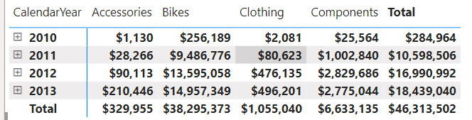
Suppose you need a measure that calculates the difference between the product categories in the order they are sorted in the visual. Implementing this as a regular DAX measure is a challenge. Yet, if we had a way to work with the cells in the visual, we can easily find a way to get this to work. Ideally, this would work similar in Excel, but DAX doesn’t know about relative cell references. However, visual calculations kind of do.

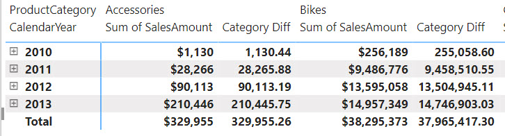
Let’s right-click on the visual and select “New calculation”. Alternatively, click the visual and then click the “New calculation” ribbon button in the Home ribbon. In the visual-level DAX formula bar, enter the following formula:

Category Diff = [Sum of SalesAmount] - PREVIOUS([Sum of SalesAmount], COLUMNS)

The Category Diff measure computes the difference between the current “cell” and the cell for the previous category. For example, for Bikes it will be $9,486,776-$28,266 (Accessories value).

The Good

As you can see, visual calculations can simplify aggregate-level metrics. Notice the use of the PREVIOUS function which is one the new DAX functions specifically designed for visual calculations. Notice also that the PREVIOUS function has additional arguments and one of them is the AXIS argument which specifies if the function should evaluate cells positionally on columns or rows. Traditional DAX functions don’t support the AXIS arguments because they are generic and not designed to operate on a visual level.

Finally, notice that visual-level formulas can only reference fields or measures placed in the visual. This is important as you’ll see later.

The Bad

Among the various limitations, the following will cause some pain and suffering:
1. You can’t export the data of a visual that has a visual calculation.
2. Drillthrough is disabled.
3. Can format visual calculations unless the visual supports it (the matrix visual does support measure formatting).
4. Can’t apply conditional formatting.
5. Can’t change sort order.
6. Can’t use field parameters.

The Ugly

The way Microsoft advertises this feature is that it is “easier than regular DAX” and performs better. My concern is that tempted by these promises, users will abuse visual calculations, such as for creating metrics that should be implemented as regular DAX measures so that any visual can benefit from them. And not before long, such users would find themselves into an Excel-like spreadmart hell which is what they tried to avoid by embracing Power BI.

I see a similar issue with DAX implicit measures, which Power BI users create by dragging a field and dropping it on a visual. I consider them a bad practice for a variety of reasons. Microsoft apparently doesn’t share the same concern (see their comments to my LinkedIn post on the same subject here). To their point, because visual calculations can only “see” fields placed in the visual, they naturally shield the user from abusing them. Let’s give it some time and see who’s right. Meanwhile, I wish this documentation article provides best practices and guidance on when to use implicit, explicit, and visual measures, including their limitations.

Visual calculations are incredibly useful but for limited scenarios. Therefore, please use these visual calculations only when regular DAX measures will not suffice. Business metrics should be centralized and should return consistent results, no matter the reporting tool or visual they are placed in. This is important for achieving the elusive single version of truth.


Teo Lachev
Prologika, LLC | Making Sense of Data
logo

A First Look at DAX Visual Calculations: the Good, the Bad, and the Ugly

The February 2024 release of Power BI Desktop includes a preview of visual calculations. As its name suggests, a visual calculation is a visual-scoped DAX measure that works at the aggregate (visual) level.
The Good

Visual calculations make previously difficult tasks much easier. Consider the following matrix:

Suppose you need a measure that calculates the difference between the product categories in the order they were sorted in the visual. Implementing this as a regular DAX measure is a challenge. Yet, if we had a way to work with the cells in the visual, we can easily find a way to get this to work. Ideally, this would work similar in Excel, but DAX doesn’t know about relative references. However, visual calculations do (kind of).

Let’s right-click on the visual and select “New calculation”. In the visual-level DAX formula bar, enter the following formula:

Category Diff = [Sum of SalesAmount] - PREVIOUS([Sum of SalesAmount], COLUMNS)

The Category Diff measure computes the difference between the current “cell” and the cell for the previous category. For example, for Bikes it will be $9,486,776-$28,266 (Accessories value).

Notice the use of the PREVIOUS function which is one the new DAX functions specifically designed for visual calculations. Notice also that the PREVIOUS function has additional arguments and one of them is the AXIS argument which specifies if the function should evaluate cells positionally on columns or rows. Finally, notice that visual-level formulas can only reference fields or measures placed in the visual.

The Bad

Among the various limitations, the following will cause some pain and suffering:
1. A visual calculation effectively disables exporting the visual data.
2. Drillthrough is disabled.
3. Can format visual calculations unless the visual supports it (the matrix visual does support measure formatting).
4. Can’t apply conditional formatting.
5. Can’t change sort order.
6. Can’t use field parameters.

The Ugly

The way Microsoft advertises this feature is that it is “easier than regular DAX”. My concern is that tempted by that promise, users will start abusing this feature left and right, such as for creating visual calculations that can be better implemented as regular DAX measures, e.g. for summing or averaging values. And not before long, such users would find themselves into an Excel-like spreadmart hell which is what they tried to avoid by embracing Power BI.

Therefore, please use these visual calculations only when regular DAX measures will not suffice. Business metrics should be centralized and should return consistent results, no matter the reporting tool or visual they are placed in. This is important for achieving the elusive single version of truth.

Atlanta Microsoft BI Group Meeting on March 4th (Navigating Microsoft Fabric – Choosing the Right Workload for Your Needs)

Atlanta BI fans, please join us in person for the next meeting on Monday, March 4th at 6:30 PM ET. The famous Patrick LeBlanc (Guy in the Cube) will take a deep dive into the Microsoft Fabric ecosystem, from Lakehouse to Warehouses and Power BI, ensuring you can make informed decisions about your data processing needs. Your humble correspondent will help you catch up on Microsoft BI latest. CloudStaff.ai will sponsor the event. For more details and sign up, visit our group page.

Presentation: Navigating Microsoft Fabric – Choosing the Right Workload for Your Needs

Delivery: In-person

Date: March 4

Time: 18:30 – 20:30 ET

Level: Beginner/Intermediate

Food: Pizza and drinks


Agenda:

18:15-18:30 Registration and networking

18:30-19:00 Organizer and sponsor time (events, Microsoft BI latest, sponsor marketing)

19:00-20:15 Main presentation

20:15-20:30 Q&A

Overview: As businesses transition to the cloud and leverage advanced analytics, understanding the nuances of data infrastructure becomes paramount. Microsoft Fabric offers a suite of powerful tools designed to handle various data workloads, but the key to harnessing its full potential lies in understanding which tool to use and when. This session provides a deep dive into the Microsoft Fabric ecosystem, from Lakehouse to Warehouses and Power BI, ensuring that participants can make informed decisions about their data processing needs. We’ll also look at current limitations that will help guide you.

Speaker: Patrick LeBlanc is a currently a Principal Program Manager at Microsoft and a contributing partner to Guy in a Cube. Along with his 15+ years’ experience in IT he holds a Master of Science degree from Louisiana State University. He is the author and co-author of five SQL Server books. Prior to joining Microsoft, he was awarded Microsoft MVP award for his contributions to the community. Patrick is a regular speaker at many SQL Server Conferences and Community events.

Sponsor: CloudStaff.ai

PowerBILogo